NEWR – Non-potable Environmental and Economic Water Reuse Calculator: Methods & Resources
1Calculator Overview
The Non-Potable Environmental and Economic Water Reuse (NEWR) Calculator is a simple, web-based tool for screening-level assessments of source water options for any urban building location across the U.S considering onsite non-potable reuse (NPR). The goal of the calculator is to identify the most environmentally and cost-effective suite of source water options to meet non-potable needs as a function of geography, climate, building size and building type. A peer-reviewed article in the journal Water Research presents NEWR output and results interpretation across the U.S. for a wide range of building configurations.
Potential environmental impacts are estimated in NEWR using life cycle assessment (LCA) following guidelines specified by the International Organization for Standardization (ISO) (ISO, 2006). LCA integrates environmental impacts occurring not only during operation of a water reclamation system, but throughout upstream supply-chains as resources are extracted, processed, distributed and consumed. Benefits (or avoided impacts) from shifting away from reliance on centralized infrastructure to onsite NPR are also incorporated in NEWR. In addition to estimating LCA environmental indicators, NEWR also generates results for life cycle cost assessment (LCCA), a similarly comprehensive approach to approximating economic costs over the lifetime of a system (Fuller & Petersen, 1996).
The intended user for NEWR is any building designer, utility personnel or water resource professional looking to evaluate source water options for onsite NPR at a preliminary ("screening level") level of detail. NEWR is not intended to provide a detailed engineering assessment for onsite NPR systems. NEWR is recommended for users interesting in screening level environmental and cost assessments for buildings with 50 or more occupants.
2Goal and Scope
NEWR allows users to compare water availability, environmental impact and cost across four NPR source water options: mixed wastewater, graywater, air conditioner (AC) condensate and rainwater. Users select a U.S. ZIP Code and define essential characteristics of the building and NPR system(s) they will be evaluating. In addition to the source of reuse water, users can define building size and type, fixture water use efficiency and end use.
Local climate data is used to determine the potential of air conditioner condensate and rainwater to satisfy NPR demand. Local climate data are also used to determine evapotranspiration from any irrigated area. Mixed wastewater and graywater are treated in an onsite, building-scale water resource recovery facility that uses an aerobic membrane bioreactor (AeMBR) as the primary biological treatment step. All treatment systems were designed to meet safety standards for indoor NPR, which includes meeting recommended log reduction targets (LRTs) for microbial pathogens in the case of graywater and mixed wastewater.
LCA results are calculated and presented per 1 gallon of NPR water provided to the building , termed the functional unit. The functional unit provides a fair basis of comparison across source water options. Users can also view LCA and LCCA results on an annual basis. Not all source water options provide the same volume of NPR water to the building on an annual basis, and NEWR specifies the overall percentage of building NPR demand met by each source water option.
LCA and LCCA results are generated in terms of Global Warming Potential, Total Energy Demand, Fossil Fuel Depletion, Water consumption, Water Scarcity and Net Present Value. Table 1 presents brief methodological descriptions of each metric. Within the NEWR interface, results can be exported in multiple formats (PNG, JPG, PDF, SVG, CSV, XLS).
| Impact/Inventory Category | Description | Unit |
|---|---|---|
| Global Warming Potential | The Global Warming Potential impact category represents the heat trapping capacity of greenhouse gases (GHGs) over a 100-year time horizon. All GHGs are characterized as lb of carbon dioxide equivalents (CO2 eq) according to the Intergovernmental Panel on Climate Change (IPCC) 2013 5th Assessment Report (IPCC, 2013). Reported global warming potential is the sum of all GHGs released to produce the energy and materials necessary for water treatment and reuse. To see how the global warming potential impact of water reuse compares to other common activities, enter tool results into EPA's Greenhouse Gas Equivalencies Calculator . | lb CO2 eq |
| Total Energy Demand | The Total Energy Demand indicator is a cumulative inventory category that accounts for the total usage of non-renewable fuels (natural gas, petroleum, coal and nuclear) and renewable fuels (such as biomass and hydro). Energy is tracked based on the higher heating value of the fuel utilized from point of extraction, with all energy values summed together and reported on a megajoule (MJ) basis. This indicator is adapted from a method previously developed by Ecoinvent (Althaus et al., 2010). The Department of Energy's Appliance Energy Calculator can be used to contextualize the energy demand of different water reuse options. | BTU |
| Fossil Fuel Depletion Potential | Fossil Fuel Depletion Potential category captures the consumption of fossil fuels, primarily coal, natural gas and crude oil. All fuels are standardized to kg oil eq based on the heating value of the fossil fuel, according to the ReCiPe impact assessment method (Huijbregts et al., 2017). Reported fossil fuel depletion is the sum of all fossil derived energy used to produce the energy and materials necessary for water treatment and reuse. | lb oil eq |
| Water Consumption | The water consumption inventory indicator accounts for use of freshwater resources that makes water subsequently unavailable to the watershed from which it was sourced. Consumptive uses include evapotranspiration, product incorporation or discharge outside of the basin. This is a similar approach to the blue water footprint approach defined by the Water Footprint Network (Hoekstra et al., 2011). | gallons H2O |
| Water Scarcity | Water scarcity is calculated using the Available Water REmaining (AWARE) Method. Results are calculated by multiplying water consumption results by the AWARE water scarcity factor, effectively weighting water consumption by the degree of its impact. The United Nations Environmental Program Water Use in LCA (WULCA) working group developed the AWARE method to assess water consumption impacts. The AWARE score is a midpoint indicator to assess the available water remaining in a watershed after the demand of humans and aquatic ecosystems has been met (Boulay et al., 2018). AWARE scores, which range from 0.1 – 100, are calculated for individual watersheds, and aggregated at the ZIP Code, Emissions & Generation Resource Integrated Database (eGRID) subregion or country basis if necessary based on the level of geographic information known for all supply chain steps. Where AWARE water scarcity factors were not available for certain ZIP Codes, they were estimated based on the average of neighboring AWARE grid cells. The AWARE method recognizes that water consumption has greater environmental significance in areas with lower water availability. | gallons H2O deprivation |
| Cost - Net Present Value (NPV) | Cost is assessed using the NPV of system alternatives over a 30-year time horizon (Fuller & Petersen, 1996). Net present value considers capital and recurring costs, using a 5% discount rate to quantify future expenditures in current dollars. | 2016 $ |
3Calculator Scenario Selections
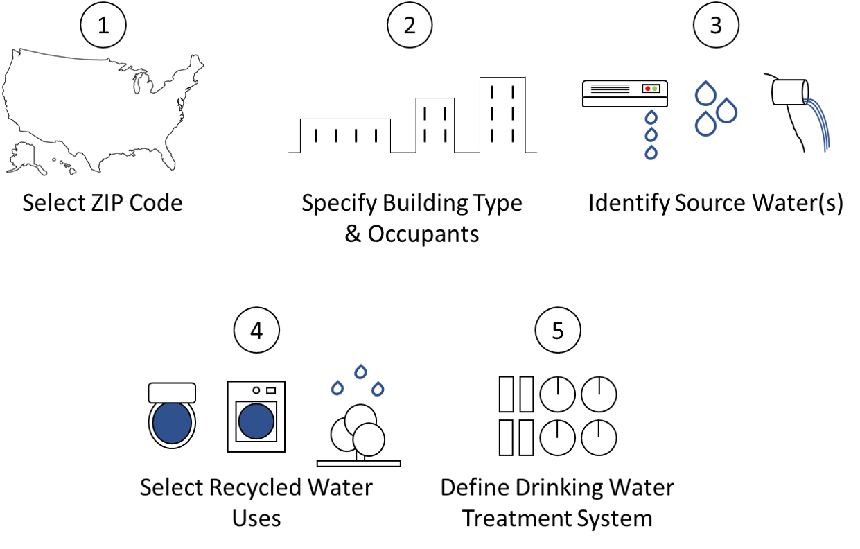
The user interface of NEWR is organized into five sections designed to guide the user in characterizing a building and selecting reuse options. The five sections are described below and illustrated in Figure 1:
- Specify ZIP Code – ZIP Code that affects all geographically dependent calculations.
- Building Characterization – General information about the type and size of the building.
- Source Water Characterization – Allows the user to define a single source or multiple sources of water, as well as the ability to define appliance characteristics.
- End Use Characterization – Characterization of how the treated water will be used within the building.
- Displaced Drinking Water – Options defining if and how drinking water costs and impacts will be offset by reuse
The calculations resulting from these user scenario selections are described in more detail in the subsequent sections.
3.1Building Characterization
Table 2 outlines the user information entered for Building Characterization. ZIP Code is used to query geographic-dependent calculation inputs while the remaining items are used to define the building water balance and modify underlying life cycle inventories.
| Data Input | Data Type | Description/Dependencies |
|---|---|---|
| Enter ZIP Code | integer (5 digits) |
|
| Select Building Type | menu |
|
| Specify Number of Building Occupants | integer (count) |
|
| Specify Number of Floors | integer (count) |
|
| Enter Total Building Footprint | integer (square feet) |
|
To define building type, the user is given the option of selecting default values (see Table 2) or inputting custom values. Building type is limited to residential, office (i.e., commercial) or mixed use (70% residential, 30% commercial). Although there are many more non-residential use categories found in typical U.S. buildings, NEWR is limited to office to provide a contrast to residential water use characteristics and to keep data input and results interpretation simple.
Default values for the number of building occupants are based on U.S. commercial and residential building survey data. Large building characteristics are based on previous evaluations of NPR systems for large buildings, where attributes were drawn from various sources (Ghimire et al., 2017, 2019; Morelli et al., 2019). To design a commercial rainwater harvesting (RWH) and air conditioner condensate harvesting (ACH) system, Ghimire et al. (2019, 2017) reviewed CBECS data on large buildings in the U.S. (EIA, 2016) to design a “typical…system in an average size commercial building sited in a large U.S. city” (Ghimire et al., 2017). Their resulting systems were designed to provide toilet flush water for buildings with 1000 occupants, a footprint of 19,600 ft2 and 4 and 19 floor configurations. Using a more regionally targeted approach, Morelli et al.'s (2019) evaluation of membrane bioreactor (MBR)-based NPR systems looked at representative buildings in San Francisco's South of Market district to define a theoretical “Large Building”, with 520 residential occupants, 590 office workers, a building footprint of 20,000 ft2 and 19 floors. To characterize smaller buildings, additional review of CBECS and U.S. Census data was performed. Of the 16,000 office buildings surveyed as part of the 2012 CBECS, 88% had fewer than 50 workers (EIA, 2016). For residential buildings, only a third of new construction in 2016 was for buildings with fewer than 30 units, down from 44% in 2010 indicating a downward trend in smaller buildings (Census Bureau, 2018).
Table 3 shows the resulting occupant number defaults. The minimum value is included to keep any user-defined custom value within a range that is both representative of actual building construction and within appropriate ranges for the NPR treatment systems selected for NEWR.
| Building Category | Number of Occupants |
|---|---|
| Large Building | 1100 |
| Medium Building | 550 |
| Small Building | 110 |
| Calculator Minimum | 50 |
3.2Source Water Characterization
Table 4 outlines the user information entered for Source Water Characterization. Input data on the source water tab determines the technology comparison used to generate results and directly impacts the water balance of the building scenario.
| Data Input | Data Type | Description/Dependencies |
|---|---|---|
| Source Water Option | menu (checkboxes) |
|
| Incorporate Thermal Recovery | menu (radio buttons) |
|
| Wastewater Collection Type | menu (radio buttons) |
|
| Building Water Use Efficiency | menu (radio buttons) |
|
Three source water options are available to generate results. One or more options may be selected simultaneously. The wastewater collection type menu option is used to specify whether mixed wastewater or source separated graywater will be collected for NPR. Wastewater type affects treatment system design, thermal recovery potential, and the quantity of water available for NPR. All treatment systems included in the calculator were designed to ensure that guidelines for indoor NPR were met (Sharvelle et al., 2017), as discussed further in Life Cycle Inventory Development.
NEWR provides users the option to capture low grade thermal energy present in either mixed wastewater or graywater. Wastewater is first put through a fine screen and is then run through a heat pump that transfers thermal energy from the influent wastewater to the building hot water heating system, with the option to displace consumption of either electricity or natural gas. Avoided burden credits, leading to reduced environmental impacts, are assigned based on the reduced fuel demand. The avoided burden approach also eliminates allocation between co-products in accordance with ISO 14044 (ISO, 2006).
Users can specify whether buildings have standard or high efficiency water use appliances. High efficiency appliances lead to a lower wastewater generation rate and lower demand for NPR water within the building.
3.3End Use Characterization
Table 5 outlines user information entered for End Use Characterization.
| Data Input | Data Type | Description/Dependencies |
|---|---|---|
| Select uses of NPR water | menu (checkboxes) |
|
Four end uses of NPR water are available for selection. One or more options may be selected simultaneously. Irrigation water demand is calculated as a function of irrigated area, and is specified as low, medium or high depending on vegetation evapotranspiration rates. The basic calculations are based on EPA's WaterSense Water Budget Tool (v 1.04) (U.S. EPA, 2020). Plant water use is defined using a unitless Plant Factor that ranges from zero to one as defined in Table 6. Plant factors relate evapotranspiration rates of a selected plant species to a reference evapotranspiration rate. Plant factors can be looked up using the online database, Water Use Classification of Landscape Species ( WUCOLS IV ) (Costello & Jones, 2014).
| Water Use Category | Plant Factor Range | Example Plants |
|---|---|---|
| Low | 0-0.35 | Yarrow (groundcover), Aloe, Bunchberry |
| Medium | 0.35-0.65 | Bermudagrass, Barberry, Sugar Maple |
| High | 0.65-1 | Kentucky bluegrass, White Birch, Loosestrife |
3.4Displaced Drinking Water Characterization
The final NEWR user input tab determines whether NPR water displaces the production, distribution and consumption of water via the centralized potable water system. Displacing potable water avoids the environmental burdens of the centralized potable water systems and serves as a primary motivation and justification for NPR. Table 7 describes default menu options on the displaced drinking water tab.
| Data Input | Data Type | Description/Dependencies |
|---|---|---|
| Does NPR Water Displace Drinking Water? | menu (radio buttons) |
|
| Select Network Leakage Rate | menu (drop down) |
|
| Define Energy Use of Drinking Water Treatment | menu (radio buttons) |
|
When the 'Custom' option is selected, an additional menu option is generated allowing users to specify individual characteristics of the drinking water treatment system that influence total energy demand. Table 8 lists water service utility characteristics and describes the available menu options. Drinking Water Treatment and Distribution describes how user selections are used to determine the electricity demand of water service provision.
| Data Input | Characteristic | Data Type | Description/Dependencies |
|---|---|---|---|
| Define Characteristics of Water Service Utility | Ease of Access | menu (dropdown) |
|
| Acquisition Efficiency | menu (dropdown) |
|
|
| Local Topography | menu (dropdown) |
|
|
| Distribution Efficiency | menu (dropdown) |
|
|
| Treatment System Energy Use | menu (dropdown) |
|
4Water Balance Calculations
4.1General Flows
Once the building has been characterized, NEWR defines the water balance in terms of sources and demand. Depending on user selections, sources can include rainwater, AC condensate, separated greywater or mixed wastewater. It is possible to define a scenario that includes rainwater, AC condensate and one wastewater flow, however separated graywater and mixed wastewater cannot be included in the same scenario, since this is not feasible for a single building. Possible demand for non-potable water can include any combination of water for toilet flushing, laundry, outdoor irrigation or other user-specified use. Mixed wastewater includes all wastewater flows, while graywater only includes flow from showers, baths and laundry as water from kitchen sinks and dishwashers are typically excluded from graywater in the U.S. (Sharvelle et al., 2013). Table 9 provides underlying per-capita supply and demand rates used for typical in-building source and demand categories. Additional calculations are required to define flow rates for rainwater and AC condensate collection on the supply side and outdoor irrigation on the demand side. Each of these are discussed individually in subsequent sections.
| Flow | Residentiala | Officeb | Mixed Usec | |||
|---|---|---|---|---|---|---|
| Std Eff | High Eff | Std Eff | High Eff | Std Eff | High Eff | |
| Demand - Non-potable | ||||||
| Toilet | 17.3 | 6.59 | 11.4 | 7.12 | 15.5 | 6.75 |
| Laundry | 11.7 | 4.87 | 0.0 | 0.0 | 8.17 | 3.41 |
| Demand - Total | ||||||
| Potable | 29.7 | 25.2 | 6.69 | 4.18 | 22.8 | 18.9 |
| Non-potable | 28.9 | 11.5 | 11.4 | 7.12 | 23.7 | 10.2 |
| Total | 58.6 | 36.6 | 18.1 | 11.3 | 46.5 | 29.0 |
| Demand - Hot | ||||||
| Hot Waterd | 19.3 | 12.1 | 3.81 | 2.38 | 14.7 | 9.17 |
| Generation | ||||||
| Greywater | 27.0 | 21.8 | 6.69 | 4.18 | 20.9 | 16.5 |
| Mixed Wastewater | 58.6 | 36.6 | 18.1 | 11.3 | 46.5 | 29.0 |
a - Standard efficiency data from DeOreo et al. (2016), high
efficiency data from Mayer et al. (2011).
b - Adapted from Morelli et al. (2019). Assume non-potable
demand is only from toilets (no laundry). Assume standard
efficiency flows are of the same proportion to high efficiency
as for residential.
c - Weighted composite of Residential (70%) and Office (30%)
d - Based on DeOreo et al. (2016), residential hot water
use is 33% of total indoor use and 57% of faucet use.
Residential hot water use therefore calculated as 33% of
total, and office hot water use calculated as 57% of potable
use, which assumes all potable use in office buildings is
attributed to faucets.
e – Graywater includes Showers, Baths and Laundry
Notes: Eff - Efficiency
4.2Source Water Characterization
Source water quality influences the type and level of treatment required for reuse. For RWH and ACH systems, source water quality was not explicitly modeled as raw water quality is suitable for direct application of disinfection unit processes. For AeMBR systems however, source water quality directly affects the level of treatment required, both to meet applicable chemical and physical water quality guidelines and to produce effluent that can be effectively disinfected. Table 10 shows chemical and physical water quality parameters assumed for source-separated graywater (which includes showers, baths and laundry) and mixed wastewater, as well as applicable effluent guidelines. Values were adapted from standard textbook values for mixed wastewater (Tchobanoglous et al., 2014) and a literature review of reuse studies (Boyjoo et al., 2013; Eriksson et al., 2002; Ghaitidak & Yadav, 2013; Li et al., 2009), as further discussed in Morelli et al. (2019). Differences in mixed wastewater strength between residential and commercial sources were not accounted for.
| Water Quality Characteristics | Influent Values | Target Effluent Quality | ||
|---|---|---|---|---|
| Mixed WW | Graywater | Both | ||
| Characteristic | Unit | Medium Strength | Low Pollutant Load with Laundry | Effluent Quality for Unrestricted Urban Use |
| Suspended Solids | mg/L | 220 | 94 | <5 |
| Volatile Solids | % | 80 | 47 | - |
| cBOD5 | mg/L | 200 | 170 | - |
| BOD5 | mg/L | 240 | 190 | <10 |
| COD | mg/L | 510 | 330 | - |
| TKN | mg N/L | 35 | 8.5 | - |
| Ammonia | mg N/L | 20 | 1.9 | - |
| Nitrite | mg N/L | - | - | - |
| Nitrate | mg N/L | - | 0.64 | - |
| Total Phosphorus | mg P/L | 5.6 | 1.1 | - |
| Chlorine Residual | mg/L | - | - | 0.5-2.5 |
4.3Rainwater Collection
The potential to use rainwater as a non-potable water source depends on the building area available for collection, rainfall rate and tank size. Therefore, in addition to total building footprint, the user is prompted to enter in the portion available for rainwater collection, which can be any value less than the total building footprint. This area is then combined with a standard collection efficiency of 75% following Ghimire et al. (2019, 2017) and a monthly rainfall time series for the user-defined ZIP Code to calculate monthly potential rainfall, as follows:
rwh_pot_month = C * bld_area_rw * col_eff * precip_month
Where,
rwh_pot_month = potential monthly rainwater
collection (gallon/month)
bld_area_rw = building footprint available for
rainwater collection (ft2)
col_eff = rainwater collection efficiency
precip_month = monthly rainfall (inch/month)
C = unit conversion coefficient (0.623)
By using monthly rainfall rather than annual rainfall, seasonal patterns can be incorporated. A shorter time step would provide greater detail but is unnecessary in this context as large rainwater collection systems are designed with a tank that is large enough to buffer sub-monthly variability but not so large that it is underutilized. To accomplish this, the rainwater collection tank is sized as the smaller of the maximum monthly demand and the average potential monthly rainwater collection.
Monthly rainwater data were primarily obtained from a North America Climate Dataset (Museum of Vertebrate Zoology, 2011) compiled jointly by a number of organizations, which provides average monthly precipitation, in raster form, based on data from land-based weather stations from 1950-2000. In some cases, individual ZIP Code points were outside of the clipped raster products. In these isolated cases, coverage was supplemented with satellite-based MERRA-2 data (Gelaro et al., 2017). MERRA-2 data only go back to 1980, therefore an averaging period of 1980-2000 was used for these data.
To distinguish between available rainwater, or rainfall, and snow or ice (the sum of which constitutes total precipitation), monthly precipitation data were filtered to exclude precipitation from months in which a hard freeze occurred. Although similar analyses have used frost free months as the threshold (e.g., the Federal Energy Management Program's Rainwater Availability Map (Loper & Stoughton, 2019)), this tends to exclude months in which minimal frost occurs, which may not limit rainfall availability. Instead, we use presence of a hard freeze, defined as four or more continuous hours of 28°F or less, to exclude precipitation data from that month. Typical Meteorological Year 3 (TMY3) data were used to identify hard freeze months (Wilcox & Marion, 2008). TMY3 data are statistical representations of hourly meteorological conditions over a typical year for 1021 stations across the continental U.S. They are based on long-term weather data (1991-2005 for TMY3) and are intended for solar and building design purposes. Presence/absence of a hard freeze was summarized by month for each station, and monthly spatial rasters were created using inverse distance weighting interpolation. These rasters were overlaid upon monthly precipitation rasters and precipitation from months in which a hard freeze occurred was removed. The resulting lookup table provides monthly rainfall time series by ZIP Code .
4.4AC Condensate Harvesting
AC condensate is produced by AC systems as they remove moisture from air during the cooling process. Fundamentally, the amount of condensate produced is the difference between the moisture content of the air entering the air handling unit (AHU) and the moisture content of the air leaving the AHU. This difference depends on outdoor air relative humidity, indoor air relative humidity, and the amount of outdoor air introduced into the system.
Within the Calculator, condensate generation potential is calculated in two steps. First, following an approach developed and field verified by others (Lawrence et al., 2010; 2012) a model was created to calculate condensate potential in gallons per cubic foot per minute of outside air (gallons/cfm) as a function of geography. This quantity represents the maximum amount of condensation that could be produced from a cfm of outside air introduced to an AHU operating at standard indoor temperature and humidity. In this case, the temperature and humidity leaving the AHU are assumed to be 55°F and 90%, based on typical ranges identified by (Glawe, 2013) and Lawrence et al. (2010). It is calculated on an hourly timestep as follows:
Qt = Aρo,t ΔHRt / B
where,
Qt
= maximum theoretical hourly yield at time t
(gal/cfm (per hr))
A = 60 (min/hr)
ρo,t
= density of outside air at time t (lb
dry air/cf)
ΔHRt
= difference between outdoor and indoor humidity ratio at time
t (lbwater/lbdry air)
B = 8.35 (lbwater/gallonwater)
ρo = Cp/RTt
where,
C = 0.0625 (lb m3/kg ft3)
p = atmospheric pressure, 101,325 (Pa)
R = gas constant, 287.05 (J/kg K)
Tt
= temperature at time t (K)
ΔHRt = HRo,t - HRi = D [(Pwo,t /(Pa - Pwo,t )) - (Pwi /(Pa - Pwi ))]
where,
HRo,t
= outdoor humidity ratio at time t (lb
water/lbdry air)
HRi
= indoor humidity ratio, constant (lbwater/lb
dry air)
D = 0.62198 (psychometric constant)
pwo,t
= water vapor partial pressure of outside air at time
t (psi)
pwi
= water vapor partial pressure of inside air, assumed constant
(psi)
pa
= atmospheric pressure, 14.696 (psi)
pwo,t = pwso,t RHt
where,
pwso,t
= water vapor saturation pressure of outside air at time
t (psi)
RHt
= relative humidity at time t (%)
pwi = pwsi RHi
where,
pwsi
= water vapor saturation pressure of indoor air leaving the
AHU at 55°F (psi)
RHi
= relative humidity of indoor air leaving the AHU, 90 (%)
pws = Ee(77.345 + 0.0057T - 7235 / T) / T8.2
where,
pws
= water vapor saturation pressure (psi)
E = 0.000145 (psi/Pa)
T = temperature at time t for outside air,
or 285.9 (55°F) for inside air (K)
The model was run using hourly TMY3 data (Wilcox & Marion, 2008). Hourly model output was summarized by month for each station, and monthly spatial rasters were created using inverse distance weighting interpolation. The resulting lookup table provides monthly condensation potential time series by ZIP Code .
To calculate the total volume of condensate generated each month, the lookup value for monthly condensate generation per outdoor air (gal/cfm) is multiplied by the amount of outdoor air required for a given scenario. The amount of outdoor air is calculated using inputs for building occupancy, area and number of floors and assuming the building HVAC system adheres to NSI/ASHRAE Standard 62.1 (ANSI/ASHRAE, 2010), which requires a minimum ventilation rate of 5 cfm/person and 0.06 cfm/ft2.
4.5Outdoor Irrigation
Outdoor irrigation water demand depends on several factors, including the area to be irrigated, the types of plants being irrigated, and evaporative demand. The approach used to calculate outdoor irrigation demand is based on EPA's WaterSense Water Budget Tool (v 1.04) (U.S. EPA, 2020) using the following general equation:
Q = 0.6233ETo A(PF / IE)
where,
Q = irrigation water demand (gal/month)
ETo
= reference evapotranspiration (in/month)
A = irrigated area, user-defined (ft2)
PF = plant water use factor (0 to 1)
IE = irrigation efficiency (%)
The user can enter the irrigated area for high, medium or low water use plant types to capture differences in vegetation transpiration rates. To simplify groupings, it is assumed that high, medium and low plant water use factors are 0.75, 0.5 and 0.25 based on general ranges provided in the Water Use Classification of Landscape Species Database (Costello & Jones, 2014). An irrigation efficiency of 75% is assumed based on the recommended range in the California Water Budget Workbook (CDWR, 2017). Effective precipitation was not considered in the calculation, leading to a conservative (higher) estimate of irrigation water demand.
Average monthly reference evapotranspiration data for the contiguous U.S. was obtained from the satellite-based MERRA-2 (Gelaro et al., 2017). Average monthly datasets were generated from the most recent 30-year time period, which at the time of download was 1989-2018. The resulting lookup table provides monthly reference evapotranspiration time series by ZIP Code .
5Life Cycle Assessment
LCA is a methodology used to quantify the environmental impact(s) of a given product or process from cradle-to-grave (ISO, 2006). To provide a uniform basis for comparison of different systems in an LCA, a common reference unit based on the function of the systems must be defined. This common basis, or functional unit, is used to normalize the inputs and outputs of the LCA. Results of the LCA are subsequently expressed in terms of this functional unit. The functional unit used as the basis of comparison in NEWR is the supply of 1 gallon of NPR water . All LCA studies involve four main steps:
- Define the goal and scope of the analysis
- Develop the life cycle inventory
- Calculate life cycle impact assessment results
- Results interpretation
Sections 2 defines the goal and scope of this analysis. Life cycle inventory (LCI) data describes material and energy inputs required to provide the functional unit. For example, in the case of wastewater treatment systems LCI data include infrastructure materials, electricity consumption, chlorine, process emissions, etc. Inventory indicators such as cumulative energy demand and water consumption track the use of specific materials throughout the life cycle of the product system, providing proxy indicators for environmental impact.
LCI data also include pollutant emissions to land, air and water. Characterized life cycle impact assessment (LCIA) categories such as global warming potential (GWP) sum pollutant emissions across a products life cycle and standardize them to a common unit (e.g. kg CO2 equivalents) to estimate potential impacts of producing or using a given product. Most LCA studies calculate several environmental indicators to try and gain a comprehensive view on product system impacts.
Figure 2 depicts a system diagram of the NPR study system showing multiple source water options, treatment processes and end use delineations. Material, chemical and energy inputs are used throughout the system and reflect environmental burdens associated with resource extraction (mining), transportation, material processing and manufacturing, product use and disposal. A unique aspect of LCA studies is their ability to quantify such impacts across a products supply-chain, and to place them on a standard basis. The system diagram also indicates NPR end use options that can displace the need for potable water production and consumption.
Avoided burdens are critical for an understanding of the environmental performance of NPR systems. Including the avoided burdens of potable water treatment or hot water heating more fully captures the benefits of decentralized reuse. Negative impact results indicate that impacts from onsite practices are less than the impacts of services (avoided burdens) they replace.

Because of the complexity inherent in such an analysis, results interpretation is included as an explicit step in conducting an LCA study. Due to uncertainty inherent in both the LCI and applied LCIA characterization factors it is not possible to state with complete certainty that differences in potential impacts for two systems are significant differences. Users are cautioned not to interpret small differences in Calculator results as significantly different. Comparative results can be determined with a greater confidence than absolute results for one system since all systems use similar background LCI data sources for common energy and material processes (as described in Section 7.4) as well as the same LCIA characterization factors.
5.1Life Cycle Inventory Development
This section describes the systems being modeled in the LCI, a summary of key environmental flows and scaling techniques used to modify base LCIs to reflect user scenario definitions. Download the full underlying model .
5.1.1Rainwater Harvesting and Air Conditioner Condensation Harvesting Development
The RWH and ACH systems are adapted from a previous LCA of commercial RWH systems for NPR in multi-story buildings (Ghimire et al., 2017). The original systems were designed according to American Rainwater Catchment Systems Association specifications for supply of toilet and urinal flush water in a four-story building serving 1000 employees. The original design was for a demand of 2653 m3/yr (1920 gpd) and included components required for collection, storage, disinfection and distribution of rainwater. Several updates to the inventory were necessary to fit within the goal and scope of this project, including an update to disinfection processes and scaling of certain system components to better reflect systems designed for different levels of non-potable demand.
UV and chlorine disinfection processes were revised to meet roof runoff LRT guidelines – log reduction of 3.5 – for enteric bacteria (Sharvelle et al., 2017) and chlorine residuals. AC condensate does not have its own LRT as it has no source for human enteric pathogen contamination. However, a management plan is necessary to minimize growth of opportunistic bacteria (Sharvelle et al., 2017). To be conservative, we assumed ACH systems included the same UV and chlorine disinfection processes as RWH systems.
To adapt the remaining components of the original LCI to user-defined conditions, components were scaled in various ways. Table 11 explains the scaling approach for each component of the original LCI. Scaling factors and scaling factor equations are applicable to both RWH and ACH systems, as both use similar background LCIs. The ACH LCI does not include a vortex filter, as there is no need to remove rooftop sediment and debris from the ACH inflow.
| Component | Parts Description | Scaling Approach |
|---|---|---|
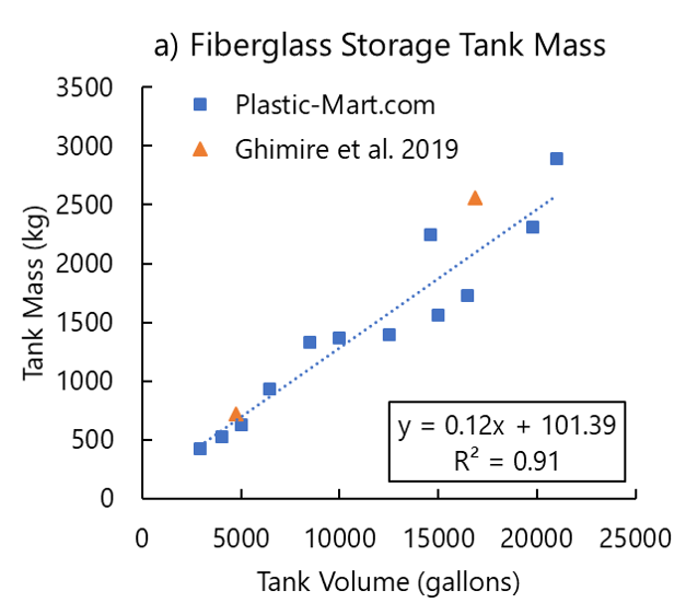
| Storage Tanks | main fiberglass storage tank, HDPE day tank | Tank mass scaled according to volume, see Figure 3 |
| Miscellaneous Components | filters, pumps, valves, sensors, pressure tank, UV light chamber | Number of components scaled according to the integer of the ratio of modeled demand to design demand |
| Disinfection | liquid chlorine, UV electricity | Constant dosage, no scaling |
| Distribution Piping | distribution piping | Original design pipe length multiplied by (1) the ratio of modeled building footprint to design building footprint and (2) the ratio of the modeled number of floors to design number of floors |
| Distribution Energy | pumping electricity | Value assumed to be 0.2 kWh/m3 for buildings greater than 4 stories, 0.1 kWh/m 3 for buildings of 4 stories or less |
Based on results of the (Ghimire et al., 2019), material associated with the main storage tank was the largest contributor to all impact categories except eutrophication potential and metal depletion (LCIA categories not covered in the Calculator). Based on preliminary scenario testing of the Calculator, the high-density polyethylene (HDPE) day tank was also one of the largest infrastructure contributors to all impact categories, especially when used for smaller buildings with few people. Therefore, to provide accurate impact results at all scales, these tank material masses are scaled based on specific water balance components. Following Ghimire et al. (2019), the main storage tank for RWH (or ACH) system is sized as the smaller of the maximum monthly demand and the average potential monthly rainwater collection (or average potential monthly condensation potential). Also following Ghimire et al. (2019), the day tank is sized as 25% of the average daily volume supplied by the RWH (or ACH) system. Tank material mass is then calculated as a function of volume using the regressions illustrated in Figure 3.

The remaining infrastructure components, not including distribution system, are scaled in a stepwise fashion using an integer scaling factor with a minimum value of one. Chemicals and electricity required for disinfection are constant across flow rates, per unit volume treated.
5.1.2Aerobic Membrane Bioreactor
The AeMBR system is the treatment option available for onsite NPR of mixed wastewater or graywater. The AeMBR model in the Calculator is adapted from an LCA performed of various treatment options designed for the onsite NPR of mixed wastewater or separated graywater (Morelli et al., 2019). The AeMBR system includes screening, an aerated equalization basin, the aerated biological reactor with submerged membrane unit (membrane bioreactor), disinfection processes in the form of ultra-violet (UV) radiation and chlorination, as well as a separate distribution system for treated water.
The treatment system was designed to meet LRTs for viruses, protozoa and bacteria to minimize human health risks. LRTs are higher for mixed wastewater, due to increased pathogen concentrations. Log reduction values (LRVs) were assigned to individual treatment processes based on unit type and dose, in the case of disinfection processes. Details of LRV assignments and their relation to LRTs can be found in Morelli et al. (2019). A free chlorine residual of 1 mg/L is established to meet water reuse guidelines (U.S. EPA, 2012).
Using user-defined building characteristics, the base design AeMBR LCI is scaled so that the system is appropriately sized for the calculated treatment flow rate of a given scenario. To adapt base design systems from Morelli and Cashman (2019) to different Scenario flow rates in a way that isolated the effects of treatment size on system cost and environmental impact, LCI components of individual unit processes were scaled in ways that maintained original design specifications (e.g., hydraulic retention time (HRT), oxygen transfer rates, chemical dosage rates, etc.) but updated applicable dimensional line items (e.g., concrete, steel, energy, etc.). Table 12 provides detail as to how individual LCI components are modified.
| Unit Process | Parts Description | Unit | Constant/Variablea | Scaling Approach |
|---|---|---|---|---|
| Fine Screen | Electricity | kWh | Variable | Energy use equation from Harris (1982) |
| Screening Disposal | kg | Constant | Constant fraction of flow | |
| Steel | kg | Constant | Constant screen area per unit of flow | |
| Equalization | Concrete | m3 | Variable | Basin volume scaled to maintain HRT and depth to area ratio. |
| Steel | kg | Variable | Basin volume scaled to maintain HRT and depth to area ratio. | |
| Electricity | kWh | Variable | Pumping energy varied as function of flow, adherence to original design equations | |
| AeMBR | Concrete | m3 | Variable | Basin volume scaled to maintain HRT and depth to area ratio. |
| Steel | kg | Variable | Basin volume scaled to maintain HRT and depth to area ratio. | |
| Polyvinyl Fluoride | kg | Constant | Constant membrane area per unit of flow | |
| Sodium Hypochlorite | kg | Constant | Constant dose rate | |
| Electricity | kwh | Variable | Pumping energy varied as function of flow, adherence to original design equations | |
| Methane | kg | Constant | Constant fraction of flow | |
| N2O | kg | Constant | Constant fraction of flow | |
| Sludge | m3 | Constant | Constant fraction of flow | |
| UV | Electricity | kWh | Constant | Constant dose rate |
| Steel | kg | Constant | Number of units increased/decreased to maintain constant UV dose | |
| Chlorination | Concrete | m3 | Variable | Basin volume scaled to maintain HRT and depth to area ratio. |
| Steel | kg | Variable | Basin volume scaled to maintain HRT and depth to area ratio. | |
| Electricity | kwh | Constant | Constant electricity per unit of flow | |
| Sodium Hypochlorite | kg | Constant | Constant dose rate | |
| Storage | HDPE | kg | Constant | Number of units increased/decreased to maintain constant storage capacity |
| Distribution Piping | PEX and PVC Piping | kg | Variable | Original design pipe length (mass) multiplied by (1) the ratio of modeled building footprint to design building footprint and (2) the ratio of the modeled number of floors to design number of floors |
| Distribution Energy | Electricity | kWh | Variable | Value assumed to be 0.2 kWh/m3 for buildings greater than 4 stories, 0.1 kWh/m 3 for buildings of 4 stories or less |
a - Constant refers to line items that are constant per unit of flow treated. Examples include chemical dose rates, such as 3 mg of NaOCl per liter of water treated.
5.1.3Thermal Recovery
The option is available to pair the AeMBR with a thermal recovery unit process to offset onsite hot water heater energy demand of either an electricity or natural gas water heater. Only buildings with a centralized boiler will be able to utilize recovered thermal energy and justify the associated environmental benefit. The thermal recovery system consists of a heat pump used to extract thermal energy from wastewater prior to treatment, transferring that thermal energy to a building's hot water system.
The thermal recovery unit process is taken directly from Morelli et al. (2019) and has variations designed for separated graywater or mixed wastewater. The difference between the two mostly has to do with the thermal energy available for recovery; the assumed temperature of mixed wastewater is 23°C, while that of separated graywater is 30°C. Individual LCI components of the thermal recovery systems are assumed constant per unit of flow. Additional information, including energy transfer calculations and LCI description, can be found in Morelli et al. (2019).
The energy recovered by the heat pump can be used to offset the energy demand of hot water heating (see Table 9 for per capita hot water demand flows). Hot water heating can be accomplished using either an electric hot water heater or a natural gas hot water heater. Although the thermodynamic calculations used to quantify the total energy demand of the two are the same, the impact associated with that energy use (or offset) varies by energy type and geography. Emission factors for natural gas are derived from the National Renewable Energy Laboratory (NREL) U.S. LCI database for combustion in an industrial boiler (NREL, 2019).
5.1.4Drinking Water Treatment and Distribution
NEWR includes an option for users to incorporate the impacts of displaced drinking water acquisition, treatment and distribution from shifting to onsite NPR. NEWR takes a simplified approach to modeling drinking water treatment by using a base model for water treatment and distribution and allowing the user to customize the inputs for energy demand based on a literature review of drinking water treatment and distribution. Because drinking water systems are complex, direct and mechanistic modeling of electricity demand is infeasible within the scope of NEWR. Instead, results from an extensive literature review were used to define ranges for water acquisition, treatment and distribution energy demand and identified major factors that influence each value. A user-defined estimate of total network leakage is then used to adjust impacts associated with the entire drinking water model (base model plus energy demand). The user is therefore able to use local knowledge to customize the estimated energy demand of their drinking water system, all while staying within realistic ranges.
The water treatment LCI model is originally based on the Greater Cincinnati Water Works (GCWW) Richard Miller Treatment Plant (Xue et al., 2019). The data in the GCWW model were adjusted to reflect a typical U.S. average potable water treatment system, which includes source water acquisition, flocculation, sedimentation, conditioning, gaseous primary disinfection, fluoridation, and addition of sodium hypochlorite to establish a residual. Underlying electricity LCI information is based on the eGRID subregion resource mix as determined by the user-selected ZIP Code. The system boundaries for drinking water displacement in NEWR include water losses during distribution to the consumer. Default water loss is an estimated 18.7 percent loss of potable water to the consumer during delivery and an additional 0.3 percent loss of fresh water during the treatment process (Xue et al., 2019). AWARE water scarcity factors (recommended AWARE100 non-irrigation) are applied to displaced source water acquisition according to ZIP Code (Boulay et al., 2018).
The first step in defining displaced drinking water impacts and costs is to select a network leakage rate. Leakage loss has the effect of requiring additional acquisition, treatment and distribution per unit of delivered water. Research has shown that energy requirements of leakage loss are roughly proportional to the volume of leakage, and can account for up to 25% of distribution energy requirements (Scanlan & Filion, 2015). Typical water loss during distribution ranges between 10% and 30% of pumped potable water (Fiut & Patience, 2013). Results of an AWWA survey indicate that losses are less than 20% for 82% of survey respondents (Friedman & Heaney, 2009). The tool allows users to select a representative water loss for their region of either 10%, 19% or 30%, with a default of 19%. This choice affects the entire potable water LCI, increasing extraction, chemical and energy requirements throughout the water treatment life cycle.
Electricity demand of potable water acquisition, treatment and distribution is determined based on the 25th and 75th percentile of case-study data identified in the literature. Figure 4 presents a box plot of electricity demand for the three stages of drinking water provision, differentiating between groundwater and surface water acquisition. Using 25th and 75th percentile values reduces the effect of outliers, which lead to atypically high values. The following five characteristics of water service utilities – (1) water resource type, (2) acquisition efficiency, (3) local topography, (4) distribution efficiency and (5) treatment system energy use – are used to estimate the electricity demand of drinking water service provision.
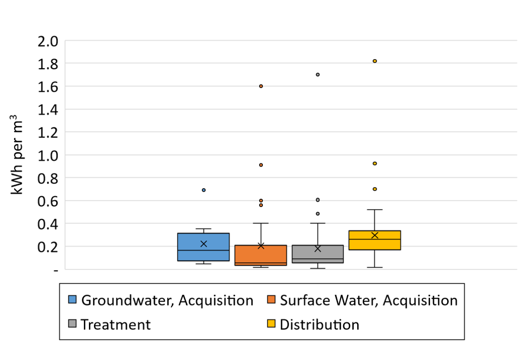
Default values are populated for each characteristic using either locally-specific or average values. Default values for water resource type and topography are calculated based on the ZIP Code selection. Options are provided for the user to either increase or decrease the default electricity demand associated with each characteristic. Regardless of user selections, the electricity demand of individual stages of drinking water service provision are bounded by the interquartile range pictured in Figure 4 and listed in Table 13 below.
To calculate total electricity demand, each of the six characteristics is assigned a point value that ranges from 0 to 5. Zero corresponds to the first quartile of case-study electricity demand while five corresponds to the third quartile. The average point value of all six characteristics is used to look up the associated electricity value in Table 13. This approach allows users to customize electricity demand associated with avoided potable water service while restricting possible outcomes to a pre-defined range.
| Drinking Water Treatment Stage | Low Electricity Demand ---------->High Electricity Demand | |||||
|---|---|---|---|---|---|---|
| Case-Study Quartiles | Q1 | Q1-Median | Median | Median-Q3 | Q3 | |
| Point Bins | 0-1 | 1-2 | 2-3 | 3-4 | 4-5 | |
| Source Water - Acquisition | Groundwater | 0.08 | 0.12 | 0.16 | 0.23 | 0.29 |
| Surface Water | 0.04 | 0.05 | 0.06 | 0.11 | 0.16 | |
| Treatment | 0.06 | 0.07 | 0.09 | 0.14 | 0.20 | |
| Distribution | 0.17 | 0.22 | 0.26 | 0.30 | 0.33 | |
| Total Energy | Groundwater | 0.31 | 0.41 | 0.51 | 0.67 | 0.82 |
| Surface Water | 0.27 | 0.34 | 0.41 | >0.55 | 0.69 | |
Source water acquisition refers to the process of getting water from a surface water or groundwater resource to the drinking water treatment facility. As a simplification the tool relies upon the assumption that generally it is more energy intensive to pump groundwater than it is to pump surface water resources. Deeper wells necessarily require greater static lift and therefore pumping energy. This general trend is supported by the boxplot in Figure 4 and EPRI's assertion that to provide drinking water from groundwater resources requires an approximate 30% increase in electricity demand relative to surface water (EPRI, 2002). The Calculator relies on county level data from the United States Geological Survey (USGS) (Dieter et al., 2018) to look up the fraction of potable water that is provided by each source water type (groundwater or surface water). The tool's default setting estimates the average electricity demand of source water acquisition using a weighted average of the local mix of groundwater and surface water. The user can also increase or decrease the default estimate of electricity demand within the Calculator. Doing so will either add or subtract 2.5 points from the default value assigned based on ZIP Code leading to maximum and minimum point values of five and zero, respectively. Although source water type and quality also influence the level of treatment required, adequate information are not available to incorporate these characteristics into the Calculator drinking water LCI. The user also has the option of setting a specific acquisition efficiency (point values: low =5, average=2.5, high=0). Acquisition efficiency is intended to represent piping distance, pump efficiency, friction loss or any other aspect of the acquisition network that will affect electricity consumption during water extraction and conveyance to the drinking water treatment plant. The average point value of water resource and acquisition efficiency is used to look up the corresponding electricity demand in Table 13.
Treatment system energy demand can also be customized. User can specify average, low or high electricity demand. Treatment system energy demand is based on the complexity of the drinking water treatment facility and is typically a function of source water quality. A treatment system with low energy demand is more representative of minimal treatment and simple disinfection processes, whereas a facility with high energy demand is likely to include advanced filtration and disinfection processes. Desalination plants are not included in this analysis. The default is set to average (point value equals 2.5).
Distribution efficiency is intended to represent factors such as friction loss (old rough pipes), pump efficiency, reservoir placement and management, to name a few. Distribution efficiency is not associated with ZIP Code and is set at the median value by default (point value equals 2.5). Users have the option to increase or decrease electricity demand based on their understanding of their location's distribution efficiency or as part of a sensitivity analysis.
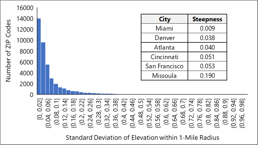
Local topography affects distribution electricity requirements, with hillier areas requiring more pumping energy (deMonsabert & Liner, 1998; Kavvada et al., 2016). A default pumping energy requirement is looked up based on ZIP Code selection and the topographical characteristics (referred to here as “steepness”) of that region relative to other regions of the United States. Steepness is calculated by estimating the variability of elevation surrounding a given ZIP Code. To perform the calculation, elevation data in raster format and at a resolution of 100 meters were obtained for Alaska, Hawaii and the conterminous U.S. (USGS 2012a, 2012b, 2012c). Next, the standard deviation of all raster pixels within a 1-mile radius of each ZIP Code location was calculated. This results in the frequency distribution illustrated in Figure 5, where roughly ~1/3 of ZIP Codes have a standard deviation of surrounding elevation values (steepness) of less than or equal to 0.02, ~1/3 of ZIP Codes have a steepness between 0.02 and 0.05, and ~1/3 of ZIP Codes have a steepness of greater than 0.05. Accordingly, point values of 1, 2.5 and 4 were assigned to each of these ranges, respectively. Using these delineations, average steepness values for a sample of major cities is also included in Figure 5, showing that Miami is considered to have low steepness, Denver and Atlanta to have moderate steepness, and Cincinnati, San Francisco and Missoula to have high steepness.
Population density was considered as an additional factor that can affect LCI quantities per unit of delivered potable water. Filion (2008) suggests that population density does influence distribution electricity consumption, but that this effect is limited to approximately 10% of total electricity demand for a given sewer configuration. Population density was ultimately excluded due to limited data availability and the relatively small potential effect on total electricity demand of drinking water service provision per unit of delivered water.
6Life Cycle Cost Assessment
The equation below shows the NPV calculation (Fuller & Petersen, 1996) used to estimate life cycle costs of operating each NPR technology over a 30-year period. The NPV method allows one-time, periodic and annual costs to be assessed on a consistent basis that considers the time-value of money using a 5% real discount rate.
Net Present Value = ∑ (Costx / (1 + i) x)
where:
NPV (2016 $) = Net present value of all costs and revenues
necessary to construct and operate the wastewater treatment
facility
Costx = Cost in future year x
i (%) = Real discount rate
x = number of years in the future
To facilitate the calculation of NPV within the Calculator itself, cost factors were developed using an Equation based on the frequency and timing of expenditures (Table 14). The unit price of electricity and natural gas are escalated over the 30-year analysis period, using escalation factors originally developed for California (Lavappa et al., 2017). Escalated energy prices are reflected in the Table 14 cost factors.
| Cost Description | Units | Cost Timing | NPV Cost Factor |
|---|---|---|---|
| Capital Cost - Year 1 Only | 2016 $ | Year 1 | 1.00 |
| Annual Cost – Electricitya | 2016 $/yr | Annual | 17.3 |
| Annual Cost - Natural Gasa | 2016 $/yr | Annual | 20.5 |
| Annual Cost - All Other | 2016 $/yr | Annual | 16.1 |
| Equipment Replacement - 5 year lifespan | 2016 $/replacement | Replace at Lifespan | 3.68 |
| Equipment Replacement - 6 year lifespan | 2016 $/replacement | Replace at Lifespan | 3.13 |
| Equipment Replacement - 7 year lifespan | 2016 $/replacement | Replace at Lifespan | 2.92 |
| Equipment Replacement - 8 year lifespan | 2016 $/replacement | Replace at Lifespan | 2.52 |
| Equipment Replacement - 9 year lifespan | 2016 $/replacement | Replace at Lifespan | 2.39 |
| Equipment Replacement - 10 year lifespan | 2016 $/replacement | Replace at Lifespan | 2.04 |
| Equipment Replacement - 11 year lifespan | 2016 $/replacement | Replace at Lifespan | 1.97 |
| Equipment Replacement - 12 year lifespan | 2016 $/replacement | Replace at Lifespan | 1.91 |
| Equipment Replacement - 13 year lifespan | 2016 $/replacement | Replace at Lifespan | 1.85 |
| Equipment Replacement - 14 year lifespan | 2016 $/replacement | Replace at Lifespan | 1.80 |
| Equipment Replacement - 15 year lifespan | 2016 $/replacement | Replace at Lifespan | 1.51 |
| Equipment Replacement - 16 year lifespan | 2016 $/replacement | Replace at Lifespan | 1.48 |
| Equipment Replacement - 17 year lifespan | 2016 $/replacement | Replace at Lifespan | 1.46 |
| Equipment Replacement - 18 year lifespan | 2016 $/replacement | Replace at Lifespan | 1.44 |
| Equipment Replacement - 19 year lifespan | 2016 $/replacement | Replace at Lifespan | 1.42 |
| Equipment Replacement - 20 year lifespan | 2016 $/replacement | Replace at Lifespan | 1.40 |
| Equipment Replacement - 21 year lifespan | 2016 $/replacement | Replace at Lifespan | 1.38 |
| Equipment Replacement - 22 year lifespan | 2016 $/replacement | Replace at Lifespan | 1.36 |
| Equipment Replacement - 23 year lifespan | 2016 $/replacement | Replace at Lifespan | 1.34 |
| Equipment Replacement - 24 year lifespan | 2016 $/replacement | Replace at Lifespan | 1.33 |
| Equipment Replacement - 25 year lifespan | 2016 $/replacement | Replace at Lifespan | 1.31 |
| Equipment Replacement - 26 year lifespan | 2016 $/replacement | Replace at Lifespan | 1.30 |
| Equipment Replacement - 27 year lifespan | 2016 $/replacement | Replace at Lifespan | 1.28 |
| Equipment Replacement - 28 year lifespan | 2016 $/replacement | Replace at Lifespan | 1.27 |
| Equipment Replacement - 29 year lifespan | 2016 $/replacement | Replace at Lifespan | 1.26 |
| Equipment Replacement - 30 year lifespan | 2016 $/replacement | Replace at Lifespan | 1.00 |
a – Annual electricity and natural gas costs have a higher cost factor than other annual costs because energy prices are assumed to increase at a rate that exceeds the standard inflation rate applied to all other annual material costs.
Total capital cost of individual treatment processes is the sum of unit process costs, direct costs, and indirect costs. Unit process costs include equipment capital expenditures and installation cost. Direct costs represent costs required to integrate individual unit processes within the larger NPR treatment system. Indirect costs include additional expenditures such as professional services, profit, and contingency costs. Direct costs were estimated by applying direct cost factors to unit process costs. Indirect costs were estimated by applying indirect cost factors to the sum of unit process and direct costs plus estimated interest during construction (Equation). An interest rate of 1.7% was used in the analysis, and represents the 2017 interest rate from California's Clean Water State Revolving Fund (CWB, 2018).
Ic = ∑ (Unit Process Costs + Direct Costs + Remaining Indirect Costs) x TCP x (ir / 2)
where:
IC (2016 $) = Interest paid during
construction
Unit Process Costs (2016 $) = Total unit process equipment and
installation cost
Direct Costs (2016 $) = Total direct costs
Remaining Indirect Costs (2014 $) = Indirect costs, including
miscellaneous items, legal costs, engineering design fee,
inspection costs, contingency, and technical
TCP = Construction period, 3 years based on CAPDETWorks™
default construction period (Hydromantis, 2014)
ir = Interest rate during construction, %
Total annual cost is the sum of operation and maintenance labor, material, chemical and energy purchases. The cost of equipment replacement is included in material cost and considers the expected lifespan of individual system components.
6.1 Cost Data Summary
Unit costs are scaled as described in the Life Cycle Inventory Development Section for use in the the LCCA. Original unit costs for RWH and ACH systems are from Ghimire et al. 2019. Original unit costs for the MBR treatment systems are from Morelli et al. 2019. The NEWR Background Model implements cost scaling and compiles LCCA results.
6.1.1 RWH and ACH System Costs
The equipment necessary to collect and disinfect rainwater and air conditioner condensate is similar for systems of comparable scale. The water collection system for both source waters includes storage tank, day tank, bag and floating filters, piping and a water level control system. Rainwater collection systems have an additional vortex filter to deal with roof debris. Distribution systems include a pump and pressure tank. Both UV and chlorine disinfection are included for both source waters. Recurring costs associated with electricity use and consumable products such as chlorine and UV bulbs are also included in the cost estimate. Direct and indirect cost factors, described above, are used to estimate additional costs associated with system design, installation, and integration of relevant system components.
Cost factors were applied to bare construction cost to estimate expenditures on maintenance materials and labor. Cost factors of 2.5% and 5% were applied to tanks and mechanical and electrical equipment, respectively. Regression equations were used to estimate operation labor requirements (hours/year) for disinfection unit processes. A labor rate of $50 per hour was applied to estimate annual operation expenditures. No additional operations labor, beyond maintenance, were included for the RWH and ACH collection systems. Administrative and laboratory labor costs are not included for RWH and ACH systems.
6.1.2 AeMBR System Costs
System configurations are similar for AeMBR treatment systems processing either graywater or mixed wastewater. Table 12 lists many of the basic components of the AeMBR treatment system. Infrastructure costs for each unit process include major pieces of mechanical equipment, concrete tank installation (where applicable), excavation and consumable goods (e.g. membrane, chemicals, UV bulbs). Direct and indirect cost factors, described above, are used to estimate additional costs associated with system design, installation, and integration of relevant system components. Major pieces of equipment for each unit process are listed below:
- Fine Screen: Redundant fine screens
- Equalization Basin: Tank, floating aerator
- AeMBR: Tank, blowers, air distribution piping and diffusers, membrane unit, permeate pump and sludge pump
- Chlorination: Tank and chemical injector
- UV: Redundant UV units
- Treated effluent storage: Tanks
- Graywater collection system: Piping
Cost factors were applied to bare construction costs to estimate expenditures on maintenance materials and labor. Cost factors of 1.5%, 5% and 11% were applied to tanks, mechanical and electrical equipment and the AeMBR unit process, respectively. Regression equations were used to estimate hourly operations labor requirements for each unit process. A labor rate of $50 per hour was applied to estimate annual operation expenditures. Administrative and laboratory labor costs are also included.
7Geographic Datasets
One of the main goals of the Calculator is to determine how geography influences the selection, design and environmental impacts of non-potable reuse options. Spatial coverage for utility rates and emissions factors were obtained for all 50 U.S. States so that values could be queried based on ZIP Code. Download all ZIP Code-specific data , with the exception of monthly time series of rainfall, condensation potential, and reference evapotranspiration.
7.1 Drinking Water Utility Rates
Drinking water utility rates were obtained from the American Water Works Association (AWWA) 2019 Water and Wastewater Rate Survey (AWWA, 2019), which includes 2018 rates from 234 large utilities across 42 states. Although there are far more than 234 water utilities across the U.S., the AWWA Rate Survey is the most comprehensive and up-to-date source of water utility rates available and has coverage for many large cities.
Rates were assigned to ZIP Codes based on city name and the user-defined building type. For ZIP Codes in cities not included in the rate survey, national medians were used. For mixed use buildings, an average of residential and commercial rates was used. Table 15 shows the rates assigned according to building type, as well as national median rates.
| Building Type | Rate Category | National Median ($/1000 gallons) |
|---|---|---|
| Residential | 5/8-inch Meter, Residential (3,740 gal/month) | $4.00 |
| Commercial | 2-inch Meter, Commercial/Light Industrial (374,000 gal/month) | $6.25 |
| Mixed Use | Average | $5.13 |
7.2 Electric Utility Rates
Electricity utility rates were obtained from a database compiled by NREL (NREL, 2017). The database consists of residential and commercial electric utility companies and rates organized by ZIP Code. User-defined building type (commercial, residential or mixed use) is used to query the appropriate rate, with mixed use calculated as an average of the commercial and residential rate. For many ZIP Codes, multiple providers and rates are available. In these cases, an average of the rates is calculated. If no data are available for a given ZIP Code, a national median is used. National median electricity rates are $0.11/kWh and $0.12/kWh for commercial and residential rates, respectively.
7.3 Natural Gas Prices
Natural gas rates were obtained from the U.S. Energy Information Administration (EIA), which publishes average rates by state but not ZIP Code (EIA, 2019). Rates were therefore assigned by state and range from $7.62 to $38.88 per thousand cubic feet.
7.4 Emission Factors
Emission factors within the Calculator were generated by applying the cumulative inventory or LCIA characterization factors described in Table 1 to the LCI factors. The regionalized cradle-to-distribution to consumer electricity emission factors use the resource mix as defined by the U.S. EPA's eGRID data from 2018 (U.S. EPA, 2018). Underlying LCI data for energy production and generation is largely taken from sources within NREL's U.S. LCI database (NREL, 2019). The U.S. LCI is a publicly available governmental database for many commodity materials and background energy and transport factors. AWARE water scarcity factors were aggregated at an eGRID subregion geographic-level for the electricity emission factors. Other background infrastructure data such as transport, virgin plastic resin production and converting are from the U.S. LCI database and originally provided by sources such as the American Chemistry Council (American Chemistry Council, 2011). The ecoinvent database , a private LCI database with data for many unit processes, was utilized when U.S.-based processes did not exist in the NREL database (Ecoinvent, 2010). For background material and fuel water scarcity and electricity factors where specific supply chain locations are unknown, the U.S. aggregated AWARE water scarcity and U.S. average eGRID factors were applied, accordingly.
8Disclaimer
Although the information in this document has been funded by the United States Environmental Protection Agency under EPA Contract No. EP-C-15-010 to Pegasus Technical Services, Inc., it does not necessarily reflect the views of the Agency and no official endorsement should be inferred.
9Source Data
10Additional Resources
NEWR Journal Article
– Water Research
Peer-reviewed publication presenting results from the NEWR
tool. Describes environmental impact and life cycle cost of
NPR across a range of source waters, building-scales and
geographies.
San Francisco Onsite Non-Potable Reuse Case Study
– Sustainability
Peer-reviewed publication describing human health, economic
and environmental trade-offs of several onsite NPR options,
using a large building in San Francisco as a hypothetical
case study.
San Francisco Onsite Non-Potable Reuse Case Study
– Full EPA Report
A detailed analysis of the original case study scenario.
Includes full supporting documentation and detailed
descriptions of modeling approaches and assumptions.
EPA's Onsite Non-Potable Water Reuse Research
webpage
A landing page describing EPA's onsite non-potable research
projects.
11Example Scenario
11.1 Starting Page
This section provides a narrative example of NEWR functions and output including data input and results interpretation. The example is based on a large, mixed-use building in San Francisco's South of Market District. In addition to this example, helpful information can be found throughout NEWR by clicking on the information icon ⓘ for individual data entry inputs and results.
NEWR's home screen (Figure 6) provides a brief description of the tool's scope and allows the user to enter any five-digit ZIP Code associated with one of the 50 U.S. states. The example ZIP Code is 94105.

11.2 Building Characterization
The Building Characterization tab ( Figure 7) allows the user to specify basic aspects of building use and configuration. The intent of NEWR is for users to select options that correspond to an existing or planned building in their region of interest. It is possible to select unrealistic building configurations and users should seek out existing designs or realistic standards as the basis of scenarios they investigate. For example, it is possible to select a number of occupants that would exceed fire code-based occupancy standards for a given floor area and use. Some guidelines that could be used to develop realistic building configurations include:
- According to the National Apartment Association the average floor area of individually metered mid- and high-rise apartments was 889 square feet (ft2) in 2019. U.S. Census data tabulated by the National Multifamily Housing Council indicates that the average occupancy of U.S. apartments is 1.85 individuals per unit, indicating that average floor space per occupant in U.S. apartments is approximately 480 ft2.
- As of 2010, the average floor space per occupant in U.S. residences was 800 square feet when including single-family homes.
- Building safety regulations dictate minimum floor area requirements per occupant for specific building uses. The typical minimum floor area requirement for office buildings is 100 ft 2 per occupant.
- Guidance from a corporate real estate advisory firm indicates that as of 2017 average floor area per office worker was approximately 150 ft2, down from 225 ft2 in 2010. Large offices typically range from 200-400 ft2. Collaborative workspaces are denser, allocating between 60 and 110 ft2 per worker.
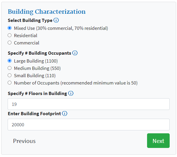
The presented example is based on a large, mixed-use building with 1,100 occupants. The building has 19 stories, each with a footprint of 20,000 ft2.
11.3 Source Water Characterization
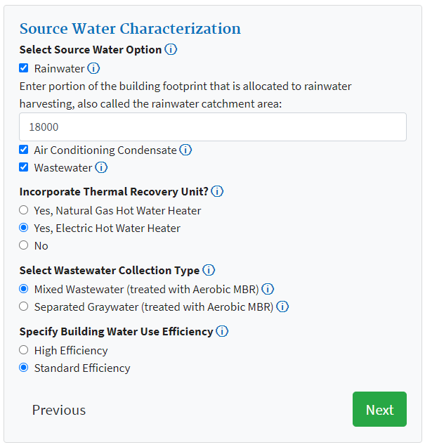
The Source Water Characterization tab ( Figure 8) allows users to select the source waters they wish to evaluate, the building's water use efficiency and whether or not thermal energy is recovered from reused wastewater.
In the example scenario all three potential sources of NPR water are selected for comparison. For rainwater, collection is assumed to take place over 18,000 ft2, slightly less than the total building footprint of 20,000 ft 2. Rainwater collection area can be any value greater than zero and less than the building's footprint. Because wastewater is selected as a source water, NEWR provides options to choose the wastewater type and whether or not thermal energy is recovered from the incoming wastewater prior to treatment. These options would disappear if wastewater is unchecked as a source water option.
In this example we selected mixed wastewater for comparison to rainwater and AC condensate. We also selected the option to evaluate a thermal recovery unit that harvests thermal energy from the mixed wastewater to supplement energy used by the electric hot water heater. Natural gas and electric hot water heaters have different environmental impacts based on their fuel source(s) and efficiency. Lessening their use through thermal recovery will alter net environmental impact results depending on water heater type. The example assumes standard per capita water use efficiency, which impacts the building's water balance and demand for NPR water.
11.4 End Use Characterization
The End Use Characterization tab ( Figure 9) allows the user to select NPR applications within their building. Check boxes can be used to select among toilet flushing, laundry, outdoor irrigation and 'other' uses. All NPR options are selected in this example scenario.
For outdoor irrigation, three water demand categories are provided that correspond to transpiration rates associated with different plant types. In the example scenario, we assume that the building has 5,000 ft2 of irrigated planted area. The high water use category is filled in to reflect irrigation of turf grass and its high water demand. The 'other' use type is available for buildings with other end uses that are suitable for water treated to non-potable standards, such as a water feature or a cooling tower. In the example scenario, we added an additional water demand of 1000 gpd.

The Displaced Drinking Water tab ( Figure 10) allows users to specify whether treated NPR water displaces water that would otherwise have been provided by the local drinking water system. Displacing drinking water provides environmental credits to the onsite water reuse system(s) by avoiding centralized drinking water treatment and distribution. When including the displaced drinking water credit, the results in NEWR represent the net change in environmental impact when transitioning to an onsite water reuse system for non-potable applications. If users want to see the full impact of onsite treatment, without avoided drinking water impacts, 'no' should be selected when asked 'Does Recycled Water Displace Drinking Water'. 'Yes' was selected for the example scenario. In some limited situations, application of an avoided drinking water treatment credit may be inappropriate; for example, if untreated surface water not from a centralized municipally treated source is currently being used for landscape irrigation.
Because 'Yes' was selected, the user is required to specify a network leakage rate and the estimated energy demand of drinking water treatment. Because of the importance of drinking water displacement to net environmental impacts, a range of options are provided to give a sense of the range of potential results associated with realistic differences in energy demand for drinking water service provision. If users have no particular insight into the operation of local utilities, default values should be selected as a starting estimate. The 'Lower' and 'Higher' 'Energy Demand' options can be used as a sensitivity analysis to understand the effect on net LCA results. The range is based on data from actual drinking water utilities and is explained in greater detail in the Drinking Water Treatment and Distribution Section. Basic research into your local utility and comparison with the data provided in the Drinking Water Treatment and Distribution Section can help guide 'Custom' selections that are more representative of your location.
For the example scenario, the minimum network leakage rate of 10% was selected based on the presence of active leak detection and pipeline replacement programs in San Francisco. To represent the energy demand of San Francisco's drinking water system, a custom scenario was developed using the following selections:
- Ease of Access: San Francisco's drinking water comes from Hetch Hetchy Reservoir and other distance surface water resources. The 'more difficult access' option was selected to reflect the size and complexity of the water acquisition system.
- Acquisition Efficiency: was set to 'high' to reflect the predominance of gravity-based flow in the acquisition piping network.
- Local Topography: was set to 'more steep' based on the hilliness of downtown San Francisco and the corresponding pump energy requirement. For a more flat city, such as Denver CO, this input could be set to 'less steep'.
- Distribution Efficiency: was set to 'high' to reflect a modern distribution system with a well-managed monitoring and maintenance program.
- Treatment System Energy Use: While the city does rely on distant water resources, the cleanliness of these water resources limits the need for filtration and other energy intensive treatment processes. As a result, 'low' was selected from the Treatment System Energy Use drop-down menu. If there is uncertainty in system energy demand, a range of energy inputs should be examined to develop an understanding of their impact on final results.
Click the 'Calculate' button and the NEWR tool will generate results.

11.5 ZIP Code Data
Figure 11 presents ZIP Code data for the entered building scenario. Additional results can be accessed by clicking on the appropriate tab at the top of the results screen. The 'Show data entered' button provides a summary of the input values selected for the current result run. Monthly water balance data is summarized in the left-most table. Regional input values used in the cost analysis and LCA results are listed in the upper right corner of the screen. A pie chart lists the fuel sources associated with the scenario's regional electricity mix.
Central California's electricity grid is relatively low carbon compared to many other U.S. regions. Natural gas is the predominant electricity fuel, providing 45% of the regions power. Solar, hydropower, nuclear and wind energy are the next most utilized fuels meeting between 15% and 7% of the state's electricity needs, respectively. Both electricity and water supply rates are well above the national averages. Natural gas prices are in the middle of the range of prices seen across the country. The water scarcity factor for this area of California is 1.84, which indicates that there is 1.84 times less water remaining per area compared to the world average.

11.6 Water Availability & Demand
Water Availability and Demand results ( Figure 12) are available on the tab immediately to the right of ZIP Code Data. Two results views, 'By Source Water Type' and 'Combined Source Water Types', are available for selection. Figure 12 presents 'Combined Source Water Type' results, where the monthly water available from rainwater, AC condensate and mixed wastewater are presented as a stacked column. Monthly non-potable demand is presented for each month and is met if the height of a stacked bar exceeds the height of the trendline.
The availability of mixed wastewater considerably exceeds monthly non-potable demand. This will typically be the case unless onsite irrigation or other consumptive uses of NPR water are significant. San Francisco has a Mediterranean climate that is characterized by warm, dry summers and cool, wet winters. This climate type is particularly poor for AC condensate generation due to low relative humidity during months when air conditioner use is common. AC condensate generation is not clearly visible in Figure 12. Hovering over the bar for an individual month shows a list of availability and demand for that period. This data indicates that condensate generation peaks at 8,100 gallons during the month of August, satisfying just under 1% of non-potable demand. Rainwater is primarily available between October and March, peaking at 42,000 gallons during the month of January. The high-rise configuration of the building used in the example scenario would not be expected to yield significant quantities of rainwater due to the large number of occupants within a small building footprint.
Clicking on the hamburger icon in the upper right corner of the results figure provides several options for downloading the figure and its underlying data. Similar export options are available on all results tabs.
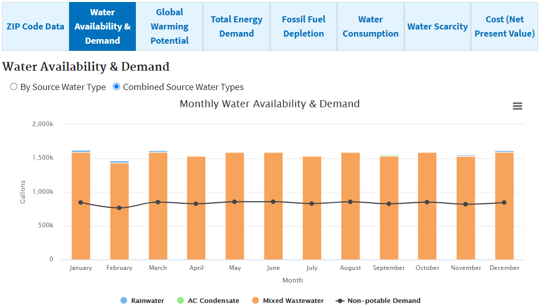
11.7 Environmental Results
Clicking on the Global Warming Potential tab pulls up the results presented in Figure 13. All six of the remaining results tabs have a similar format with two radio buttons allowing users to toggle between results per gallon of recycled water delivered and annual results that present total annual impacts for each source water type. Figure 13 presents GWP results in lb CO2-equivalents per gallon of recycled water delivered.
The magnitude of the avoided product credit for the mixed wastewater system is considerably greater than that for the rainwater or AC condensate systems, leading to a negative global warming potential impact (i.e. net reduction) for the mixed wastewater treatment system. This large environmental credit is attributable to electricity production avoided by thermal energy recovery. If the same data inputs are selected, but thermal energy recovery is turned off, then the avoided product credit for each source water option is identical because they are displacing the same quantity of drinking water on a per gallon basis. This change in inputs would shift the relative comparison between source water types, indicating that in the absence of thermal recovery, impacts would be greatest for the wastewater treatment system.
For the rainwater and AC condensate systems, infrastructure is the largest source of global warming potential impact. This is partially due to the seasonal nature of both source water types and low utilization of the installed infrastructure during seasonal lulls. Operation of the wastewater treatment system is more energy intensive but that system uses material inputs more efficiently per gallon of water provided.
Results of an LCA analysis are best used to draw comparative conclusions between alternative options with a similar or equivalent output. The NEWR tool aligns the scope of source water alternatives to ensure a fair comparison. Caution should be used when utilizing NEWR LCA results for other purposes or for comparison to other LCA analyses, as system boundaries and assumptions may be different.
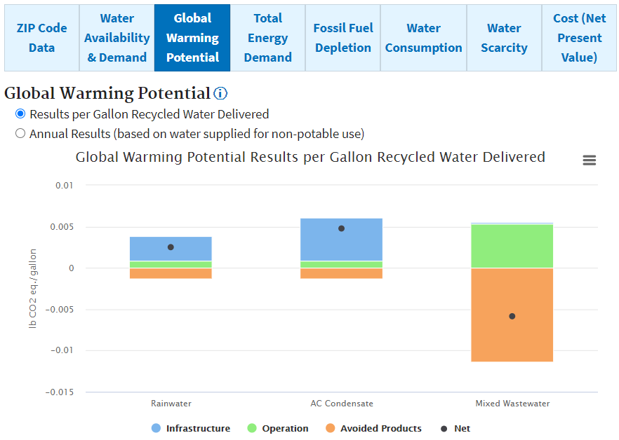
Selecting the annual results option presents the cumulative, net impact of delivering the quantity of each source water produced annually. An example of this result format is presented in Figure 14 for the water consumption indicator. Water consumption results are presented in million liters per year. Next to the label for each source water option we see the fraction of non-potable demand met that is contributing to the pictured impacts.
Rainwater, AC condensate and mixed wastewater respectively provide 2%, 0.4% and 100% of non-potable demand in the example scenario. Annual impacts presented in Figure 14 therefore represent drastically different quantities of source water. It is important to keep this in mind when interpreting annual results. On a per gallon basis, water consumption, which is net negative, is nearly identical for all source water options as it is dominated by avoided potable water production and distribution.
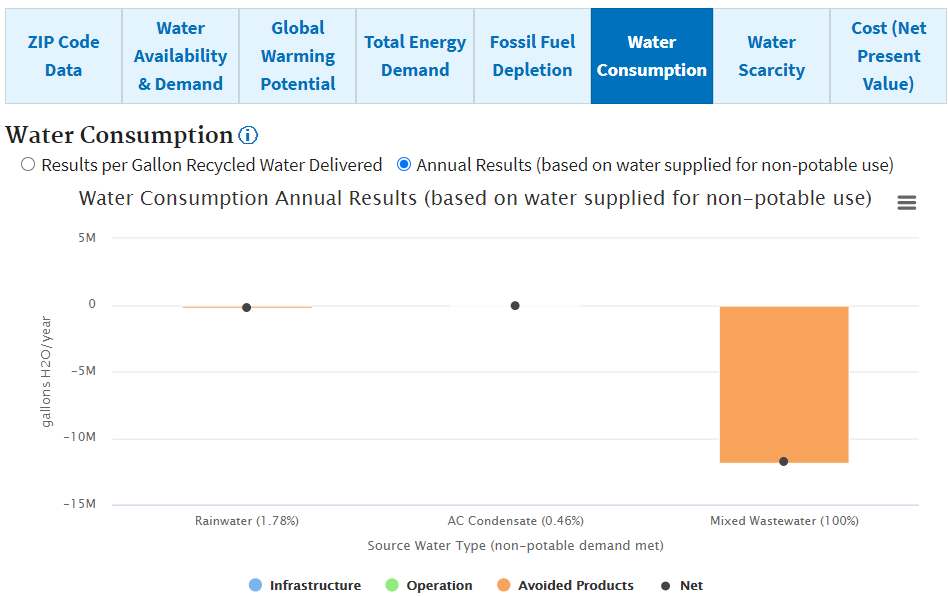
11.8 Cost Analysis Results
Figure 15 presents results of the life cycle cost analysis on a per gallon basis. Net cost per gallon over the life cycle of each system ranges from $0.0005 per gallon for the mixed wastewater treatment system (when considering avoided costs) to $0.055 and $0.078 per gallon for the rainwater and AC condensate systems, respectively.
Avoided product credits represent the avoided expense of purchasing potable drinking water and avoided electricity or natural gas costs when thermal recovery is selected. Results show that on a per gallon basis, the mixed wastewater MBR has a NPV per gallon that is similar to the avoided cost of purchasing potable water. Costs per gallon to produce NPR water from rainwater and AC condensate systems are considerably greater than the equivalent cost of potable water, which ranges from around $2 to $45 per 1000 gallons of water across the country (AWWA, 2019). Infrastructure costs are substantial for both rainwater and AC condensate systems due largely to inefficiencies in establishing a building-wide reuse infrastructure for what can be relatively small monthly flows of reuse water. Fixed annual costs associated with the operation and maintenance of each system, such as filter replacement and pump maintenance, considerably increase prices per gallon treated at low flowrates. Refer to the Life Cycle Cost Assessment Section for more information on included costs or the Full Background Model to access underlying cost data.

12List of Acronyms
| Acronym | Definition |
|---|---|
| AC | Air conditioner |
| ACH | Air conditioner condensate harvesting |
| AeMBR | Aerobic membrane bioreactor |
| AHU | Air handling unit |
| AWARE | Available Water REmaining |
| AWWA | American Water Works Association |
| BOD5 | 5-day biochemical oxygen demand |
| CBECS | Commercial buildings energy consumption survey |
| cBOD5 | Carbonaceous 5-day biochemical oxygen demand |
| cf | Cubic feet |
| CO2 | Carbon dioxide |
| COD | Chemical oxygen demand |
| eGRID | Emissions & Generation Resource Integrated Database |
| EIA | U.S. Energy Information Administration |
| FDP | Fossil fuel depletion potential |
| ft2 | Square feet |
| GCWW | Greater Cincinnati Water Works |
| GHG | Greenhouse gas |
| gpd | Gallons per day |
| GWP | Global warming potential |
| HDPE | High-density polyethylene |
| HRT | Hydraulic retention time |
| IPCC | Intergovernmental Panel on Climate Change |
| ISO | International Organization for Standardization |
| K | Degrees Kelvin |
| kg | kilogram |
| kWh | Kilowatt-hour |
| lb | pound |
| LCA | Life cycle assessment |
| LCCA | Life cycle cost assessment |
| LCI | Life cycle inventory |
| LCIA | Life cycle impact assessment |
| LRT | Log reduction target |
| m3 | Cubic meter |
| MBR | Membrane bioreactor |
| MERRA-2 | Modern-Era Retrospective analysis for Research and Applications, Version 2 |
| mg/L | Milligram per liter |
| mg N/L | Milligrams of nitrogen per liter |
| mg P/L | Milligrams of phosphorus per liter |
| MJ | Megajoule |
| NEWR | Non-Potable Environmental and Economic Water Reuse Calculator |
| NPR | Non-potable reuse |
| NPV | Net present value |
| NREL | National Renewable Energy Laboratory |
| Pa | Pascal |
| psi | Pounds per square inch |
| RWH | Rainwater harvesting |
| TED | Total energy demand |
| TKN | Total Kjeldahl nitrogen |
| TMY3 | Typical meteorological year 3 |
| USGS | United States Geological Survey |
| U.S. LCI | United States Life Cycle Inventory Database |
| UV | Ultraviolet |
| WULCA | Water Use in LCA |
| WW | Wastewater |
| yr | year |
13References
Althaus, H.-J., Bauer, C., Doka, G., Dones, R., Frischknecht, R., Hellweg, S., Humbert, S., Jungbluth, N., Köllner, T., Loerincik, Y., Margni, M., & Nemecek, T. (2010). Implementation of Life Cycle Impact Assessment Methods . Data v2.2 (2010). (p. 176). Ecoinent Centre, Swiss Centre for Life Cycle Inventories.
American Chemistry Council. (2011). Cradel-to-Gate LCI of Nine Plastic Resins and Two Polyurethane Precursors . Franklin Associates, a Division of ERG. http://plastics.americanchemistry.com/LifeCycle-Inventory-of-9-Plastics-Resins-and-4-Polyurethane-Precursors-Rpt-Only
ANSI/ASHRAE. (2010). ANSI/ASHRAE Standard 62.1-2010 Ventilation for Acceptable Indoor Air Quality .
AWWA. (2019). 2019 Water and Wastewater Rate Survey. American Water Works Association.
Boulay, A., Bare, J., Benini, L., Berger, M., Lathuillière, M. J., Manzardo, A., Margni, M., Motoshita, M., Núñez, M., Pastor, A. V., Ridoutt, B., Oki, T., Worbe, S., & Pfister, S. (2018). The WULCA consensus characterization model for water scarcity footprints: Assessing impacts of water consumption based on available water remaining (AWARE). The International Journal of Life Cycle Assessment, 23, 368–378. https://doi.org/10.1007/s11367-017-1333-8
Boyjoo, Y., Pareek, V. K., & Ang, M. (2013). A review of greywater characteristics and treatment processes. Water Science and Technology, 67(7), 1403–1424. https://doi.org/10.2166/wst.2013.675
CDWR (California Department of Water Resources). (2017). Water Budget Workbook. http://www.water.ca.gov/wateruseefficiency/landscapeordinance/
Census Bureau, U. S. (2018). Characteristics of New Housing. U.S. Census Bureau; January 2020. https://www.census.gov/construction/chars/
Costello, L. R., & Jones, K. S. (2014). WUCOLS IV: Water Use Classification of Landscape Species . California Center for Urban Horticulture, University of California, Davis. http://ucanr.edu/sites/WUCOLS/
CWB (California Water Boards). (2018). Financial Assistance Funding—Grants and Loans—Clean Water State Revolving Fund (CWSRF) . https://www.waterboards.ca.gov/water_issues/programs/grants_loans/srf/index.html
deMonsabert, S., & Liner, B. L. (1998). Integrated Energy and Water Conservation Modeling. Journal of Energy Engineering, 124(1), 1–19. https://doi.org/10.1061/(ASCE)0733-9402(1998)124:1(1)
DeOreo, W. B., Mayer, P., Dziegielewski, B., & Kiefer, J. (2016). Residential end uses of water, version 2 (Executive report). Denver, CO: Water Research Foundation.
Dieter, C., Linsey, K., Caldwell, R., Harris, M., Ivahnenko, T., Lovelace, J., Maupin, M., & Barber, N. (2018). Estimated use of water in the United States county-level data for 2015 (ver. 2.0, June 2018) US Geological Survey data release .
Ecoinvent. (2010). Ecoinvent data version 2.2. http://www.ecoinvent.org/
EIA. (2019). Natural Gas Annual 2019. U.S. Energy Information Agency. https://www.eia.gov/energyexplained/natural-gas/prices.php
EIA. (2016). 2012 Commercial Buildings Energy Consumption Survey (CBES) Table B2 . U.S. Energy Information Agency. https://www.eia.gov/consumption/commercial/data/2012/bc/cfm/b2.php
EPRI. (2002). Water & Sustainability (Volume 4): U.S. Electricity Consumption for Water Supply & Treatment—The Next Half Century (No. 1006787). Electric Power Research Institute.
Eriksson, E., Auffarth, K., Henze, M., & Ledin, A. (2002). Characteristics of grey wastewater. Urban Water, 4(1), 85–104. https://doi.org/10.1016/S1462-0758(01)00064-4
Filion, Y. R. (2008). Impact of Urban Form on Energy Use in Water Distribution Systems. Journal of Infrastructure Systems, 14(4), 337–346. https://doi.org/10.1061/(ASCE)1076-0342(2008)14:4(337)
Fiut, B., & Patience, M. (2013). Taking a Holistic Approach to Nonrevenue Water. Journal AWWA, 105(10), 54–59.
Friedman, K. R., & Heaney, J. P. (2009). Water Loss Management: Conservation Option in Florida's Urban Water Systems. Florida Water Resources Journal, 24–32.
Fuller, S. K., & Petersen, S. R. (1996). Life-Cycle Costing Manual for the Federal Energy Management Program (U.S. Department of Commerce NIST handbook 135; p. 210). National Instititute of Standards and Technology.
Gelaro, R., McCarty, W., Suárez, M. J., Todling, R., Molod, A., Takacs, L., Randles, C. A., Darmenov, A., Bosilovich, M. G., Reichle, R., Wargan, K., Coy, L., Cullather, R., Draper, C., Akella, S., Buchard, V., Conaty, A., da Silva, A. M., Gu, W., … Zhao, B. (2017). The Modern-Era Retrospective Analysis for Research and Applications, Version 2 (MERRA-2). Journal of Climate, 30(14), 5419–5454. https://doi.org/10.1175/JCLI-D-16-0758.1
Ghaitidak, D. M., & Yadav, K. D. (2013). Characteristics and treatment of greywater—A review. Environmental Science and Pollution Research, 20(5), 2795–2809. https://doi.org/10.1007/s11356-013-1533-0
Ghimire, S. R., Johnston, J. M., Garland, J., Edelen, A., Ma, X. (Cissy), & Jahne, M. (2019). Life cycle assessment of a rainwater harvesting system compared with an AC condensate harvesting system. Resources, Conservation and Recycling, 146, 536–548. https://doi.org/10.1016/j.resconrec.2019.01.043
Ghimire, S. R., Johnston, J. M., Ingwersen, W. W., & Sojka, S. (2017). Life cycle assessment of a commercial rainwater harvesting system compared with a municipal water supply system. Journal of Cleaner Production, 151, 74–86. https://doi.org/10.1016/j.jclepro.2017.02.025
Glawe, D. (2013). San Antonio Condensate Collection and Use Manual for Commercial Buildings. Engineering Faculty Research. https://digitalcommons.trinity.edu/engine_faculty/9
Hoekstra, A. Y., Chapagain, A. K., Aldaya, M. M., & Mekonnen, M. M. (2011). The water footprint assessment manual: Setting the global standard . Earthscan.
Huijbregts, M. A. J., Steinmann, Z. J. N., Elshout, P. M. F., Stam, G., Verones, F., Vieira, M., Zijp, M., Hollander, A., & van Zelm, R. (2017). ReCiPe2016: A harmonised life cycle impact assessment method at midpoint and endpoint level. The International Journal of Life Cycle Assessment, 22(2), 138–147. https://doi.org/10.1007/s11367-016-1246-y
Hydromantis. (2014). CAPDETWorks Version 3.0 Software: Rapid Design and Costing Solution for Wastewater Treatment Plants .
IPCC. (2013). Climate Change 2013: The Physical Science Basis. Contribution of Working Group I to the Fifth Assessment Report of the Intergovernmental Panel on Climate Change . Cambridge University Press. http://www.climatechange2013.org/images/report/WG1AR5_Frontmatter_FINAL.pdf
ISO. (2006). ISO 14044: 2006 Environmental management—Life cycle assessment—Requirements and guidelines (ISO 14044:2006(E); ISO 14044, p. 54). The International Organization for Standardization. https://www.iso.org/standard/38498.html
Kavvada, O., Horvath, A., Stokes-Draut, J. R., Hendrickson, T. P., Eisenstein, W. A., & Nelson, K. L. (2016). Assessing Location and Scale of Urban Nonpotable Water Reuse Systems for Life-Cycle Energy Consumption and Greenhouse Gas Emissions. Environmental Science & Technology, 50(24), 13184–13194. https://doi.org/10.1021/acs.est.6b02386
Lavappa, P. D., Kneifel, J. D., & O'Rear, E. (2017). Energy Price Indices and Discount Factors for Life-Cycle Cost Analysis – 2017 Annual Supplement to NIST Handbook 135 (NISTIR 85-3273-32; p. 90). National Instititute of Standards and Technology.
Lawrence, T., Perry, J., & Alsen, T. (2012). AHU Condensate Collection Economics. ASHRAE Journal; New York, 54(5), 18-20,22,24-25.
Lawrence, T., Perry, J., & Dempsey, P. (2010). Predicting Condensate Collection from HVAC Air Handling Units. ASHRAE Transactions; Atlanta, 116, 3–15.
Li, F., Wichmann, K., & Otterpohl, R. (2009). Review of the technological approaches for grey water treatment and reuses. Science of the Total Environment, 407(11), 3439–3449. https://doi.org/10.1016/j.scitotenv.2009.02.004
Loper, S. A., & Stoughton, K. M. (2019). Rainwater Harvesting Potential Maps (DE-AC05-76RL01830). U.S. Department of Energy. https://www.pnnl.gov/main/publications/external/technical_reports/PNNL-25498Rev1.pdf
Mayer, P., Deoreo, W. B., Opitz, E. M., Kiefer, J. C., Davis, W. Y., Dziegielewski, B., & Nelson, J. O. (2011). Residential end uses of water.
Morelli, B., Cashman, S., Ma, Cissy, Garland, Jay, Bless, Diana, & Jahne, Michael. (2019). Life Cycle Assessment and Cost Analysis of Distributed Mixed Wastewater and Graywater Treatment for Water Recycling in the Context of an Urban Case Study (EPA/600/R-18/280; p. 162). U.S. Environmental Protection Agency.
Museum of Vertebrate Zoology, U. of C., Berkeley, USA. (2011). North America Climate—Monthly Precipitation. Commission for Environmental Cooperation. https://www.sciencebase.gov/catalog/item/4fb55169e4b04cb937751d9b
NREL. (2017). U.S. Electric Utility Companies and Rates: Look-up by Zipcode (2017) . National Renewable Energy Laboratory. https://openei.org/doe-opendata/dataset/u-s-electric-utility-companies-and-rates-look-up-by-zipcode-2017
NREL. (2019). U.S. Life Cycle Inventory Database. www.nrel.gov/lci/
Plastic-Mart.com. (2019). Above-Ground Vertical Fiberglass Tanks.
Scanlan, M., & Filion, Y. R. (2015). Application of Energy Use Indicators to Evaluate Energy Dynamics in Canadian Water Distribution Systems. Procedia Engineering, 119, 1039–1048. https://doi.org/10.1016/j.proeng.2015.08.931
Sharvelle, S;, Ashbolt, N., Clerico, E., Hultquist, R., Leverenz, H., & Olivieri, A. (2017). Risk-Based Framework for the Development of Public Health Guidance for Decentralized Non-Potable Water Systems .
Sharvelle, Sybil, Roesner, L., & Glenn, R. (2013). Treatment, Public Health, and Regulatory Issues Associated with Graywater Reuse: Guidance Document (No. 9781934183939). WateReuse Research Foundation.
Tchobanoglous, G., Burton, F. L., Stensel, H. D., Tsuchihashi, R., Abu-Orf, M., Bowden, G., & Pfrang, W. (2014). Wastewater Engineering: Treatment and Resource Recovery (5th ed.). McGraw-Hill Education.
U.S. EPA. (2012). Guidelines for Water Reuse (EPA/600/R-12/818; p. 643). https://www.epa.gov/sites/production/files/2019-08/documents/2012-guidelines-water-reuse.pdf
U.S. EPA. (2018). Emissions & Generation Resource Integrated Database (eGRID) . U.S. Environmental Protection Agency. https://www.epa.gov/energy/emissions-generation-resource-integrated-database-egrid
U.S. EPA. (2020). WaterSense Home Specification: Water Budget Tool (v 1.04) (Version 1.04) [Excel]. https://www.epa.gov/watersense/water-budget-tool
USGS. (2012a). 100-Meter Resolution Elevation of Alaska100-Meter Resolution Elevation of the Conterminous United States. National Atlas of the United States . http://nationalatlas.gov/atlasftp-1m.html
USGS. (2012b). 100-Meter Resolution Elevation of Hawaii. National Atlas of the United States. http://nationalatlas.gov/atlasftp-1m.html
USGS. (2012c). 100-Meter Resolution Elevation of the Conterminous United States . National Atlas of the United States. http://nationalatlas.gov/atlasftp-1m.html
Wilcox, S., & Marion, W. (2008). Users Manual for TMY3 Data Sets (Revised) (NREL/TP-581-43156). National Renewable Energy Lab. (NREL), Golden, CO (United States). https://doi.org/10.2172/928611
Xue, X., Cashman, S., Gaglione, A., Mosley, J., Weiss, L., Ma, X. C., Cashdollar, J., & Garland, J. (2019). Holistic analysis of urban water systems in the Greater Cincinnati region: (1) life cycle assessment and cost implications. Water Research X, 2, 100015. https://doi.org/10.1016/j.wroa.2018.100015