
LakeCat Data Processing and Quality Assurance
Introduction
This document describes the main steps folled to develop the LakeCat Dataset as well as the quality assurance procedures to verify the integrity of LakeCat data. See the LakeCat GitHub page for the latest version of code used to develop the LakeCat Dataset. First, we will go over the processing steps then discuss the quality assurance methods used to confirm our findings.
Processing Steps
Three distinct aspects of LakeCat development are as follows:
- LakeCat Framework - This section describes the development of the geospatial framework of NHDPlusV2 lakes, their associated local catchments, and the process to hydrologically link nested catchments to allow for the calculation of full watershed metrics.
- Landscape Layers - Geospatial layers representing both natural (e.g., climate, soils, and geology) and anthropogenic (e.g., urbanization, agriculture, and dams) landscape features were then processed through the LakeCat framework to produce lake catchment and watershed summaries. This section describes the acquisition, checks, and manipulation (e.g., geographic transformations) of these layers to prepare them for processing to produce Lakecat data.
- Metric Calculation - The LakeCat framework and the landscape layers are then combined to calculate the suite of catchment and watershed metrics that make up the LakeCat Dataset. This section describes the steps used to produce both local catchment summaries and the accumulation of these summaries to produce full watershed summaries.
LakeCat Framework
Lakes that intersect with the NHDPlusV2 stream network were processed differently than those that did not intersect with this network. Specifically, lakes that intersect with the stream network already had landscape metrics calculated for them as part of the StreamCat Dataset and these data were drawn directly from those tables to populate LakeCat (see the StreamCat Dataset for documentation of StreamCat development). Lakes that did not intersect with the NHDPlusV2 stream network required the development of a custom geospatial framework (see below).
1. Determine On-Network and Off-Network Lakes
The NHDPlusV2 distributes waterbody features as shapefiles (NHDWaterbody.shp) by HydroRegion. These features contain several types of waterbody features, including lakes, wetlands, and estuaries. Waterbodies are first filtered by this waterbody type (i.e., the column named 'FTYPE' in the shapefile) to only include 'LakePond' or 'Reservoir' types. Lakes that intersect with the NHDPlusV2 stream network, fit within the NHDPlusV2 geospatial framework that was used to develop StreamCat. Catchment and watershed metrics for these lakes were drawn directly from StreamCat.
After finding on-network lakes, the remaining lakes are considered off-network lakes (Fig. 1). These waterbodies required a custom framework to create catchment boundaries to produce statistical summaries of landscape layers (e.g., land cover) that could be aggregated to full watershed summaries.
The following sections provide additional details on the processes we used to generate catchment and watershed metrics for on-network and off-network lakes.
2. On-Network Process
Below we describe the step-by-step process for finding lakes we classify as On-Network.
Step 1 - Find lakes On-Network
The process to identify on-network lakes used a series joins among tables that are available for download with the NHDPlusV2 (Fig. 1).
To begin, we determined which NHDPlusV2 waterbodies are on the NHDPlusV2 network by joining the following tables within each NHDPlusV2 HydroRegion (see code in LakeCat_function.py, NHDtblMerge function):
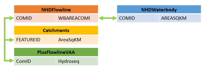
Figure 1. NHDPlusV2 table joins to find on-network lakes. NHDFlowline = attribute table of NHDPlusV2 stream network file NHDFlowline.shp, Catchments = attribute table of NHDPlusV2 catchments file Catchments.shp, PlusFlowlineVAA = NHDPlusV2 value added attribute table PlusFlowlineVAA.dbf, NHDWaterbody = attribute table of NHDPlusV2 lakes in Waterbody.shp
-
NHDPlusV2 waterbodies that are associated with NHDFlowlines through the 'WBAREACOMID' are identified through the first table join (orange to blue table join in Fig. 1). Within the stream network shapefile NHDFlowline.shp, the WBAREACOMID corresponds to the COMID in NHDWaterbody.shp (i.e., columns labeled COMIDs in NHDFlowline.shp and NHDWaterbody.shp do not correspond).
-
Join the NHDPlusV2 Catchments and NHDPlusFlowlineVAA tables to the joined tables from (1) by FEATUREID and COMID, respectively. FEATUREID in Catchments.shp corresponds to COMID in NHDFlowline.shp and PlusFlowlineVAA.dbf (orange to yellow and yellow to green table joins in Fig. 1). Using these joined tables, we group records by the waterbody COMID with the NHDtblMerge function. This grouping identifies instances where multiple stream catchments are associated with a single lake (e.g., on-network lake in Fig. 1). Within each group, we search for any FEATUREID value that is not null. For non-null FEATUREIDs, we select the FEATUREID with the lowest Hydroseq value (green table in Fig. 1) within each group. This query identifies the most downstream catchment among the catchments intersecting with a lake and is the COMID used to query watershed metrics from StreamCat. A Python dictionary holds a list of the catchment IDs that are associated with the lowest Hydroseq catchment COMID. For example, the catchments IDs in Fig. 1 that intersect with the on-network lake are stored in a list within a Python dictionary where the key of that list is the COMID of the most downstream catchment.
The remaining waterbodies are not on the stream network (i.e., they have no WBAREACOMID in the NHDFlowline.shp attribute table) and are designated as Off_Network lakes and saved as off-network.shp in the LakeCat geospatial framework. Watershed characteristics are developed for these lakes using the Off-Network Process.
Step 2 - Join associated catchments for local area 'Cat' metrics
On-network lakes are often the confluence of multiple stream segments (Fig. 2). The NHDPlusV2 connects these stream confluences within lake waterbodies with segments called ‘artifical paths’ (yellow segments in Fig. 2) and the NHDPlusV2 delineated local catchments for each of these segments (yellow polygons in Fig. 2). Local catchments for these lakes is an aggregation of all NHDPlusV2 catchments intersecting the lake. Note that not all on-network lakes are associated with multiple catchments.
The LakeCat_functions.py script creates arrays that hold the associated catchment COMIDs with the lake's most downstream catchment COMID. The same accumulation function is used to create summary statistics across all catchments associated with each waterbody, and updates catchment-level statistics to report summaries for all associated catchments to the given NHDWaterbody.
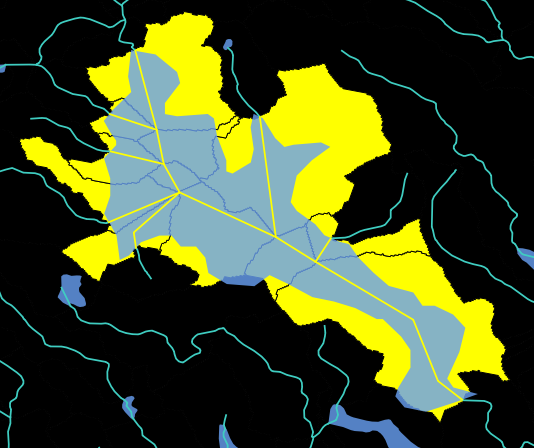
Figure 2. On-network lakes (light-blue polygon) are often the confluence of multiple flowlines (yellow lines) with associated NHDPlusV2 catchmens (yellow polygons). A local catchment summary for this lake in LakeCat is the aggregated StreamCat summary of all NHDPlusV2 catchments shown in yellow.
Step 3 - Add terminal lakes to LakeCat
NHDPlusV2 distributes a shapefile called Sink.shp with each HydroRegion. This shapefile consists of point locations of terminal flow (i.e., no outlet) within the NHDPlusV2 network, such as self-draining basins. Lakes that occur in terminal basins are not identified as on-newtork through Step 2 but can be identified with the Sink.shp shapefile. These points are attached to waterbodies through a spatial join and added to the list of on-network lakes. The 'PURPDESC' field of the point is identified as 'NHDWaterbody closed lake' (Fig. 3) and like other on-network lakes, its waterbody COMID and catchment COMID are stored to produce local catchment summaries by pulling from StreamCat data.
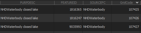
Figure 3. Attribute table of Sink.shp in NHDPlusBurnComponents
3. Off-Network Process
After finding on-network waterbodies, the remaining are moved into the off-network process to create a custom geospatial framework that will operate in similar ways to that of the NHDPlusV2 catchments and flow tables that were the basis of StreamCat.
Step 1 - Create local catchments for each off-network lake
All off-network lakes were converted from ESRI shapefiles to rasters (.TIF format) using the NHDPlusV2 flow accumulation raster as a snap raster (Fig. 4). This aligns the lake rasters with the flow accumulation raster and other rasters used in processing in NHDPlusV2. These lake rasters are used as the pour point in the ESRI Watershed tool (see makeBasins function in LakeCat_functions.py). The output of this tool provides hydrologic boundaries based on digital topography for each lake (Fig. 4).
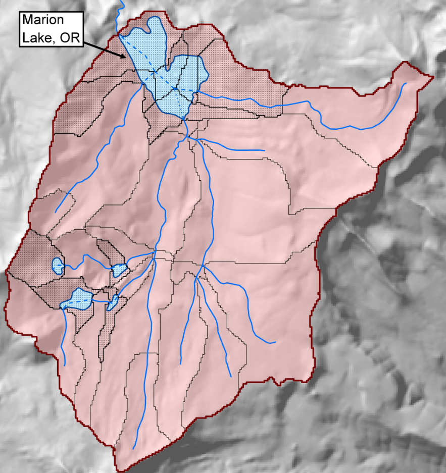
Figure 4. Example of on-network lakes and their associated catchments. On-network lakes intersect with NHDPlusV2 stream lines and often have several tributaries with separate catchments (black stippled catchments of Lake Marion). LakeCat aggregates the local catchments that intersect with each lake polygon and reports catchemnt-level statistics for these combined catchments. The set of hydrologically linked catchments that feed to Lake Marion, OR are in pink. Figure from Hill et al. (2018).
These boundaries are called ‘catchments’ for consistency with the NHDPlusV2 framework for streams. When several lakes occur in sequence, the ESRI watershed tool produces a series of nested, non-overlapping catchments, where the ID of each catchment corresponds to the raster ID of each input lake (Fig. 5).
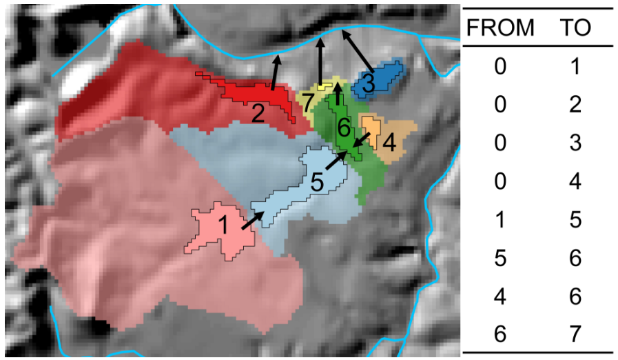
Figure 5. Example of off-network lakes (opaque with black outline) and their local catchments (semi-transparent). Numbers within lakes are unique identifiers and arrows indicate the direction of hydrologic connection among lake catchments. Hydrologic connections among lake catchments can be represented with a toplogy table. Figure from Hill et al. (2018).
Step 2 - Find flow connections between basins
A custom Python tool that shifts rasters in each of the cardinal and ordinal directions and NHDPlusV2 flow direction raster can be used to determine where connections occur between two adjacent lake catchments (see rollArray and makeFlows functions in LakeCat_functions.py for Python code to connect lake catchments). To do so, a script shifts the raster cells of each set of local catchments by one pixel distance (Fig. 6). For each shift, the script tests if the value of that shifted cell is different from the value that it holds in the unshifted raster. If different, the adjacent cell represents a possible flow connection between the two catchments. The script then tests if the flow direction raster value demonstrates that there is flow in the same direction as the direction of the shift. If both of these criteria are met, those cells are flow connected and this connection is stored in a from-to flow table (Fig. 5). The shift is done for each of the ordinal and cardinal map directions that a raster cell can be moved and all connections are recorded in a final flow connection table.
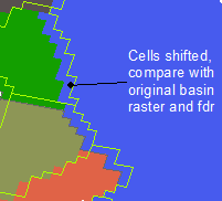
Figure 6. Cells shifted and compared with original catchment and flow direction rasters
Landscape Layers
Here we detail the steps used to process landscape layers into LakeCat.
1. Landscape Layer Acquisition
LakeCat was developed to parallel StreamCat in the numbers and types of landscape metrics. To develop the first phase of the StreamCat Dataset, we identified potential landscape metrics through a literature review. Specifically, we used several landscape metrics identified in Carlisle et al. 2009, Falcone et al. 2010, and Wang et al. 2011. Data were downloaded from online sources where available.
For the second phase of the StreamCat project, we conducted an extensive search for publically available, conterminous USA-wide landscape layers that we hypothesized could improve our representation of natural and anthropogenic watershed features. These layers included climate, groundwater usage, forest cover change (yrs. 2001-2010), atmospheric N deposition, and fish passage barriers. These data were added to this FTP site as they became available.
2. Layer Checks
The orginal characteristics of each landscape layer were documented and checked for consistency:
- Landscape Feature - Name of GIS layer used in analysis
- Description - A short description of the landscape layer (see also Data Dictionary)
- Source - From where the data were obtained, especially through personal contacts
- Original GIS Format - Original file type of landscape layer
- URL - URL from which layer was downloaded, if applicable
- Check Projection - Check the original projection of the data. Desired projection was USGS Albers Equal Area Conic Projection
- Check raster resolution - Documentation of the resolution of GIS raster, if applicable
- Check Spatial Extent - Verify that the raster covers the conterminous USA (visual check)
- Crosses CAN/MEX borders - Check whether layer extends into Canada or Mexico
- Check NoData Values - For raster layers, document the NoData values (e.g., -9999 vs. true NoData values)
- Check Units - Document the units of data layers, if applicable
- Visual Check - Opened layer in ArcGIS and visually inspected it for outliers, odd values, file corruption
3. Layer Manipulation
After documenting the original characteristics of each dataset, we then manipulated the data to standardize geospatial projections and other characteristics across layers where necessary. Data were standardized using a Python script. Manipulations, final data formats, and final data units were documented, including:
- Unit or NoData Conversion - ArcGIS raster calculator commands to convert to SI units
- Final Units - The final units of layers, if applicable
- Check range of converted values - Verify that values of final layers are within expected ranges
- Final GIS Format - The final file type of landscape layer
- Notes - Additional notes and actions that were required to standardize landscape layers
Metric Calculation
The process to calculate catchment and waterhsed metrics for on-network lakes is documented as part of the StreamCat Dataset. Data for on-networks lakes were pulled directly from StreamCat. The following section describes the process to calculate catchment and watershed metrics for off-network lakes. These metrics were combined with data from on-network lakes to produce final LakeCat data tables.
1. Zonal Statistics
The first step to create watershed metrics was to generate statistical summaries of landscape layers for each catchment. We overlaid the catchment boundaries onto landscape layers and calculated a suite of summary statistics (Table 1). The ESRI zonal statistics tool was used in a Python script to make these catchment-level summaries (see LakeCat.py at LakeCat GitHub repository).
Table 1. Example of an zonal processing results for a continuous raster type. Results differed from this example if original landscape layer was a categorical data type. Column labeled 'VALUE' was a unique ID that corresponded to delineated lake catchments.
| VALUE | COUNT | AREA | MIN | MAX | RANGE | MEAN | STD | SUM | VARIETY | MAJORITY | MINORITY | MEDIAN |
|---|---|---|---|---|---|---|---|---|---|---|---|---|
| 113210 | 12705 | 11434500 | 0 | 0 | 0 | 0 | 0 | 0 | 1 | 0 | 0 | 0 |
| 113211 | 173 | 155700 | 0 | 0 | 0 | 0 | 0 | 0 | 1 | 0 | 0 | 0 |
| 113212 | 1838 | 1654200 | 0 | 0 | 0 | 0 | 0 | 0 | 1 | 0 | 0 | 0 |
| 113213 | 1278 | 1150200 | 0 | 0 | 0 | 0 | 0 | 0 | 1 | 0 | 0 | 0 |
| 113214 | 246 | 221400 | 0 | 0 | 0 | 0 | 0 | 0 | 1 | 0 | 0 | 0 |
| 113215 | 789 | 710100 | 0 | 0 | 0 | 0 | 0 | 0 | 1 | 0 | 0 | 0 |
Zonal statistics produces statistical summaries that are stored in .dbf files. These catchment summaries must be accumulated to produce full watershed summaries from nested catchments (e.g., Fig. 5). To do so, a Python script first uses the from-to connections of nested catchments and a tree-walking algorithm to create lists (i.e., a Python numpy array) of all upslope catchments for each catchment in a network of catchments (see children and bastards functions in LakeCat_functions.py at LakeCat GitHub repo). Next, SUM and COUNT columns from the zonal statistics table are mapped to these lists so that a sum of the SUM and COUNT columns can be made for each waterhsed by looping through these catchment lists (see Accumulation function in LakeCat_functions.py at LakeCat GitHub repo). Once accumulations are made, these results are combined with data from off-network lakes and stored as comma-delimited text files (Table 2). The columns that are contained in the new file depends on the type of base landscape layer (raster, point, line) and whether the watershed metric is based on a continuous (e.g., soils) or categorical (e.g., land cover) data type. In addition, the area (km2) of catchments are calculated and appended to these tables. Finally, a column ('inStreamCat') is added to indicate whether the data originated from StreamCat (i.e., on-network lakes) or if it was generated through the LakeCat framework (i.e., off-network lakes).
Table 2. Example of an accumulated results for a continuous raster type. Results differed from this example if original landscape layer was a categorical data type.
| COMID | CatAreaSqKm | CatCount | CatSum | CatPctFull | UpCatAreaSqKm | UpCatCount | UpCatSum | UpCatPctFull | WsAreaSqKm | WsCount | WsSum | WsPctFull | inStreamCat |
|---|---|---|---|---|---|---|---|---|---|---|---|---|---|
| 19761090 | 1.2699 | 1411 | 165 | 100 | 0.0000 | NA | NA | NA | 1.2699 | 1411 | 165 | 100 | 0 |
| 22538780 | 0.6021 | 669 | 343 | 100 | 0.3744 | 416 | 0 | 100 | 0.9765 | 1085 | 343 | 100 | 0 |
| 22538782 | 0.0774 | 86 | 241 | 100 | 0.0000 | NA | NA | NA | 0.0774 | 86 | 241 | 100 | 0 |
| 22538788 | 0.1827 | 203 | 200 | 100 | 0.0000 | NA | NA | NA | 0.1827 | 203 | 200 | 100 | 0 |
| 22538790 | 0.6336 | 704 | 0 | 100 | 0.0000 | NA | NA | NA | 0.6336 | 704 | 0 | 100 | 0 |
| 22538798 | 0.2133 | 237 | 8 | 100 | 0.0000 | NA | NA | NA | 0.2133 | 237 | 8 | 100 | 0 |
3. Point Layer PctFull
LakeCat reports the percent completeness of data within each watershed (Table 2). CatPctFull and WsPctFull represent the minimum data completeness of geospatial data within the catchment and watershed metrics used in modeling (i.e., across all predictors used in the model). For example, if 50% of the area of a catchment intersected with NoData values of a geospatial layer and all other geospatial layers for that catchment were complete (100%), then the CatPctFull value reported for that catchment is 50%.
In categorical and continuous landscape layers we are able to determine if there are NoData cell values within each catchment through the return of the statistics functions ( ZonalStatisticsAsTable, TabulateArea). Each of these delivers a COUNT statistic, identifying how many cells w/in the zone hold data. This is compared with the total number of cells known to be in the zone based on the Catchment rasters attribute table to produce the percent full statistic (PctFull).
Currently, all point-level metrics (e.g., dams) that are summarized for StreamCat and LakeCat are US-only data. To account for portions of the watershed with missing data (i.e., that cross into Canada or Mexico), the borderline of the conterminous US (CONUS) is used from the TIGER line files for states (Fig. 7). See PointInPoly function in LakeCat_functions.py at LakeCat GitHub repo for code.

Figure 7. Illustration of lake catchments that cross an international border. For point data (e.g., dams), LakeCat uses the US boundary and lake catchments to calculate data completeness as a percent of the lake catchment within the US.
4. Final Tables
Final catchment and watershed metrics are calculated from the catchment and watershed SUM and COUNT columns in Table 2 with the following equations:
-
Continuous metrics - Lw = \(\sum_{c} x_c / \sum_{c} n_c~c \epsilon w\)
Lw is the mean of the continuous landscape layer for watershed w, xc is the sum of values for all pixels in catchment c with data, and nc is the number of pixels with data in catchment c, where catchment c is a member of the list of catchments that comprise watershed w (\(c \epsilon w\)).
-
Categorical metrics - Pw,i = \(100 \sum_c x_{c,i} / \sum_c n_c~c \epsilon w\)
Pw,i represents the percent of watershed w comprised of class i, xc,i is the count of pixels of class i in catchment c, and nc is the number of all pixels in catchment c, with catchment c being a member of a list of catchments within watershed w (\(c \epsilon w\)).
-
Point density metrics - Vw = \(\sum_c n_c / \sum_c \pi_c A_c~c \epsilon w\)
Vw is the density of points within watershed w, nc is the count of points within catchment c, \(\pi\)c is the proportion of area (Ac) of catchment c within the US border (Fig. 7), with catchment c being a member of a list of catchments within watershed w (\(c \epsilon w\)). Attributes tied to point or line features (e.g., dam volume) can be summarized for watershed by modifying this equation to be:
-
Point attribute metrics - Uw = \(\sum_c x_c / \sum_c \pi_c A_c~c \epsilon w\)
Uw is the sum of point feature attributes (e.g., dam volume) within watershed w per unit area of watershed w, xc is the sum of point attributes within catchment c, \(\pi\)c is the proportion of area (Ac) of catchment c within the US border (Fig. 7), with catchment c being a member of a list of catchments within watershed w (\(c \epsilon w\)).
Note that the point density and point attribute equations can be modified to summarize the density or attributes of line features within watersheds (e.g., road density as total road lengths per unit watershed area).
Final metrics are saved in a comma-delimited text file for distribution (Table 3). The first 6 columns of all LakeCat tables are:
-
COMID - Lake unique identifier that can be linked to lakes within the NHDPlusV2 NHDWaterbody.shp shapefile.
-
CatAreaSqkm - Area of catchment (km2).
-
CatPctFull - % of lake catchment that overlaps with landscape layer. Accounts for areas of NoData pixels and international borders.
-
WsAreaSqkm - Area of watershed (km2).
-
WsPctFull - % of lake watershed that overlaps with landscape layer. Accounts for areas of NoData pixels and international borders.
-
inStreamCat - Flag identifying lakes that intersected with NHDPlusV2 stream lines (value = 1) and lakes that did no intersect stream lines (value = 0). Rows with value = 1 have catchment and watershed metrics that were drawn directly from the StreamCat Dataset.
The number and types of columns after the first 6 columns can vary depending on data source and metric type
-
Cat Metrics - Suite of catchment-level metrics with 'Cat' suffix in name.
-
Ws Metrics - Suite of full watershed-level metrics with 'Ws" suffix in name.
Table 3. Example of a final LakeCat table (2006 human-related imperviousness). Results differed from this example if original landscape layer was a categorical data type.
| COMID | CatAreaSqKm | WsAreaSqKm | CatPctFull | WsPctFull | inStreamCat | PctImp2006Cat | PctImp2006Ws |
|---|---|---|---|---|---|---|---|
| 19761090 | 1.2699 | 1.2699 | 100 | 100 | 0 | 0.1169383 | 0.1169383 |
| 22538780 | 0.6021 | 0.9765 | 100 | 100 | 0 | 0.5127055 | 0.3161290 |
| 22538782 | 0.0774 | 0.0774 | 100 | 100 | 0 | 2.8023256 | 2.8023256 |
| 22538788 | 0.1827 | 0.1827 | 100 | 100 | 0 | 0.9852217 | 0.9852217 |
| 22538790 | 0.6336 | 0.6336 | 100 | 100 | 0 | 0.0000000 | 0.0000000 |
| 22538798 | 0.2133 | 0.2133 | 100 | 100 | 0 | 0.0337553 | 0.0337553 |
LakeCat - Quality Assurance
Below we move into the quality assurance steps taken for the LakeCat Dataset.
Introduction
Both the LakeCat geospatial framework and final metrics were subjected to quality assurance (QA) procedures to ensure the integrity of LakeCat data. This document describes these steps.
On-network lakes used data directly from the StreamCat Dataset and those data were, therefore, subjected to QA as part of StreamCat development. This document descibes the QA of off-network lakes. However, final LakeCat data (on- and off-network lakes combined) were subjected to final check regardless of data source (see section Final Metric Checks below).
Off-network lakes required the development of a custom geospatial framework.
FTYPE Drop
The NHDPlusV2 contains 448,512 waterbody polygons (Table 1). The first step in the LakeCat process was to remove 69,415 waterbodies that were designated as 'Ice Mass', 'Playa', or 'SwampMarsh' in the 'FTYPE' column of the waterbody shapefile attribute table. This query left 379,097 waterbodies designated as 'Lake/Pond' or 'Reservoir' for which watershed metrics could potentially be calcualted. Note that the FTYPE designations are part of the NHD and no further checks were completed to verify the accuracy of these designations.
Table 1. Numbers of waterbodies within NHDPlusV2. Total Waterbodies = FTYPE Drop + On-Network + Sink Add + Off-Network + Out-of-Bounds. Column definitions: VPU = NHDPlusV2 Vector Processing Unit; FTYPE Drop = Number of waterbodies without FTYPE 'LakePond' or 'Reservoir'; On-Network = Number of waterbodies that are linked through the WBAreaCOMI attribute to the NHDPlusV2 stream network; Sink Add = Number of waterbodies that can be added back into On-Network through the NHDPlusV2 table 'NHDBurnComponents'; Off-Network = Number of waterbodies within VPU bounds that aren't linked with WBAreaCOMI attribute; Out-of-Bounds = Waterbodies that exist spatially outside of the bounds of the VPU geometry and must be placed in the correct VPU before processing.

Sink Catchments
The query to identify on-network lakes results in 121,620 water bodies (Table 1). However, this query fails to identify lakes that occur in self-draining, terminal catchments, called “sinks” in the NHDPlusV2. Terminal or sink lakes are identified through an additional query (see Step 3 of On-Network Process above). This query added an additional 4,373 lakes to the on-network lakes table (Table 1). Numerous sink lakes were examined in a GIS to verify that they represented lakes in terminal catchments.
Off-Network Lakes
There are 250,104 off-network waterbodes in the NHDPlusV2 (Table 1). These waterbodies required a custom geospatial framework to calculate catchment and watershed metrics. Numerous catchment delineations were examined in a GIS to verify that the ESRI Watershed tool was producing catchments as expected. In addition, zonal statistics and accumulated metrics were calculated by hand for several metrics to ensure the integrity of scripted calculations.
Out-of-Bound Lakes
The NHDPlusV2 is distributed by major HydroRegion. Through the QA examinations of off-network lakes (above), we discovered several instances where lakes were placed and being distributed in the wrong HydroRegion. We developed a script to test if lakes were oustide of the geographic boundary of the HydroRegion they were distributed with. This script identified 3,000 lakes (Table 1) that we then placed in correct HydroRegions to be processed as off-network lakes.
Oversized catchments
Off-network lakes had small local catchments and full watersheds. In general, the areas of catchments and watersheds should be smaller than the NHDPlusV2 catchments that contain the lakes. We identified 326 lakes with catchments that were larger than the NHDPlusV2 catchments that contained them. However, these lake catchments were visually inspected and found to be accurate and were included in LakeCat. A list of these 326 lakes can be found in a column called 'oversized' in the attribute table of off-network.shp in the LakeCat framework.
Omitted Lakes
The number of NHD waterbodies with FTYPEs of 'LakePond' or 'Reservoir'was 379,097 (i.e., the sum of On-Network, Sink Add, Off-Network, and Out-of-Bounds lakes in Table 1). LakeCat tables deliver metrics for 378,088 lakes. Below, we account for the 1,009 waterbodies that were omitted from LakeCat.
- There were 44 lakes that extended beyond their NHDPlusV2 raster processing unit (RPU). RPUs are sub-regions within HydroRegions that are used to distribute digital elevation models (DEMs) and hydrologic derivatives of DEMs, such as flow direction rasters. It was not possible to create accurate catchment delineates for lakes that extended beyond these boundaries (Fig. 8).
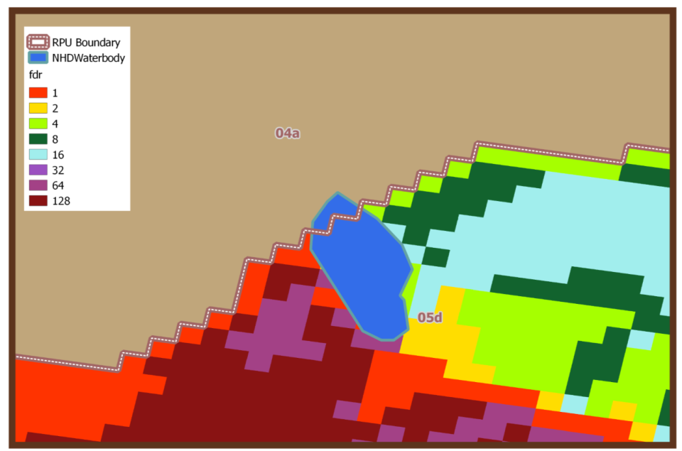
Figure 8. Example of a lake that extends beyond its RPU. Flow direction grids (fdr) cannot accurately depict watershed boundaries for these lakes.
-
A total of 939 lakes were outside of the boundary of the conterminous US. These lakes, therefore, did not overlap with NHDPlusV2 flow direction rasters that were used for catchment delineation.
-
We found 8 lakes were duplicated (i.e., same area and unique ID) within the NHDPlusV2. In each case, one of the duplicated records was removed.
COMID VPU1 VPU2 13871500 05 07 120050356 07 09 22324609 04 07 7109029 04 09 13118610 04 07 15516922 02 04 15516920 02 04 18156163 03W 08 -
9 lakes had polygons that overlapped with with other lakes, i.e., same or similar lake boundary but different unique IDs. In each case, one of the polygons was selected and one was omitted.
Figure 9. Example of a small lake that does not intersect with the centroid of the 30x30m rasters that are distributed with the NHDPlusV2.

| COMID | VPU | REASON FOR OMISSION |
|---|---|---|
| 14300071 | 10U | OVERLAPPED BY COMID 12568346 |
| 120051949 | 10U | OVERLAPPED BY COMID 120052923 |
| 167245973 | 10L | OVERLAPPED BY COMID 120053749 |
| 24052877 | 17 | OVERLAPPED BY COMID 20315924 |
| 120054048 | 17 | OVERLAPPED BY COMID 120053946 |
| 19861298 | 16 | OVERLAPPED BY COMID 24989585 |
| 162424445 | 15 | OVERLAPPED BY COMID 120053954 |
| 14725382 | 04 | OVERLAPPED BY COMID 166766632 |
| 120054030 | 18 | OVERLAPPED BY COMID 120053926 |
-
There were 9 very small lakes that did not intersect with raster centroids. Lake polygons were converted to lake rasters that matched the extent and grid spacing of NHDPlusV2 hydrologic rasters. Some small lakes did not intersect with the centroids of these rasters because of their size and position and could not be processed (Fig. 9).
COMID VPU REASON FOR OMISSION 12967474 10U DOESN'T HIT CELL CENTER 14819137 07 DOESN'T HIT CELL CENTER 14820667 07 DOESN'T HIT CELL CENTER 944040052 14 DOESN'T HIT CELL CENTER 23854057 17 DOESN'T HIT CELL CENTER 22323839 09 DOESN'T HIT CELL CENTER 15235574 08 DOESN'T HIT CELL CENTER 22700864 08 DOESN'T HIT CELL CENTER 20166532 03N DOESN'T HIT CELL CENTER
Final Metric Checks
We conducted an independent evaluation of LakeCat data by comparing LakeCat metrics to those calculated for a subset of lakes as part of the US EPA's 2007 National Lakes Assessment (NLA). The NLA method and data sources for watershed delineation and metric calculation differed from the LakeCat method but a common landscape layer was summarized between the two studies; the 2006 National Land Cover Dataset (NLCD). The two methods produced very similar estimates of percent cropland within lake watersheds, with a coefficient of determination (r-squared) of 0.91 between the 2 estimates (Fig. 3; from Hill et al. 2018). Several instances of outliers were examined and in all cases differences could be attributed to the differing methods and data sources used by LakeCat and NLA. In all instances that we examined, large LakeCat-NLA differences were due to (1) NLA merging 2 or more lake polygons (i.e., sampling occurred during a wet year and lakes were combined to reflect observed conditions) or (2) differences in hydrologic rasters used by LakeCat or NLA.
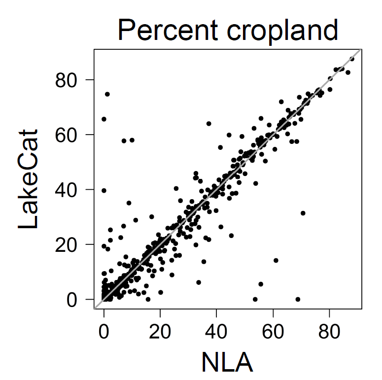
Figure 10. LakeCat versus NLA estimates of percent cropland within lake watersheds. Figure from Hill et al. (2018).