
Seagrass Data Retrieval in EDM
Estuary Data Mapper (EDM) includes submerged aquatic vegetation (SAV) in estuaries of the conterminous United States. This page explains the technical aspects of the SAV data and strategies for accessing that data in EDM.
On this page:
- Updated Submerged Aquatic Vegetation Data for Conterminous United States
- Strategy for Data Discovery, Visualization, and Download of SAV Data
- Example: Pacific Coast
- Example: Atlantic and Gulf Coast Retrievals
- Minimum Distance Filtering Added to Some Estuaries
Submerged Aquatic Vegetation Data for Conterminous United States
A time series of monitoring data related to submerged aquatic vegetation (SAV) in estuaries and some nearshore environments of the conterminous United States has been updated recently and released for public use.
The SAV data for the Pacific coast was reformatted slightly for EDM from a database published in 2018 by the Pacific Marine and Estuarine Fish Habitat Partnership (PMEP; www.pacificfishhabitat.org). Subsequently, EPA compiled SAV data from publicly available sources (generally States, Federal agencies, National Estuary Programs, or National Estuarine Research Reserve sites) for the Atlantic and Gulf coasts. EPA formatted these datasets to be as similar to the Pacific coast as possible given the constraints of available metadata. Attributes related to monitoring methods for the different sources are compiled into a table incorporated into the polygon coverage metadata as pipe-delimited records that can be extracted and parsed into a table in Excel or various open-source spreadsheet programs. The data sources used by EDM can be viewed in Seagrass Monitoring Data Sources (xlsx)
Geodatabase elements for SAV data have been exported as shapefiles for sharing via EDM. Static variables were retained in the shapefile, and time-varying attributes are provided in an associated csv file with a common link (EelgrassUID) for matching. (Note that the EelgrassUID variable name is a carryover from the Pacific Coast dataset which includes only Zostera species, while the full data set incorporating both Atlantic and Gulf Coast data includes other seagrass species as well.) One significant difference between Pacific and other coastal databases is that the PMEP database recorded absence as well as presence data from surveys, while the other surveys did not consistently record absence. Another significant difference is that the Pacific coast database is focused on Zostera (eelgrass), whereas species present in other coastal datasets are more diverse.
In general, data were compiled by “unioning” SAV polygon coverages for a given estuary across different surveys so resultant polygons may represent one year or many years of record. The latest year of record is recorded for each polygon to allow estimates of the most recent recorded extent of SAV in any monitored estuary. Maximum extent of seagrass across all years of record was also estimated. The historic sequence is recorded so that users can analyze time series if desired. Time varying data are delivered in an accompanying csv file with the following fields: EelgrassUID :Unique ID for each eelgrass feature in the feature class and Year :Year in which data were collected. The EelgrassUID can be used to join with the polygon data so that users can extract data for any year of interest to evaluate time series. In the process of simplifying polygon coverages to a common spatial resolution, some very small polygons were removed, converted to points, and saved with the original polygon attributes in a separate layer (Points2 in the menu). This helps to speed up the visualization and download process for these fine-resolution datasets.
Due to the fine-scale resolution of SAV data and the extensive spatial and temporal coverage in some systems, we had to limit user access to one estuary (or sub-estuary for a few large systems) at a time for visualization and download of polygon data to prevent long delays in response or having the system “time-out” before full retrieval. The full database for each coast is available from EPA on request for users who need to conduct more extensive analyses. Thus, the retrieval strategy for SAV data is different from the standard protocol for data discovery, visualization, and downloads of other datasets in EDM.
Strategy for Data Discovery, Visualization, and Download of SAV Data
In general, gridded, Point, and Pac Point data are retrieved for the entire viewing area. Polygon and Point2 data are retrieved for the selected ESTCODE shown in the adjacent menu and then the View automatically zooms to show the retrieved data. For the Pacific coast, select either Eelgrass (Polygon) or Eelgrass (Pac Point). For the Atlantic or Gulf coasts, select either Eelgrass(Polygon), Eelgrass(Point), or Eelgrass(Point2). The Point2 dataset represents polygons too small to see (e.g., single pixel size).
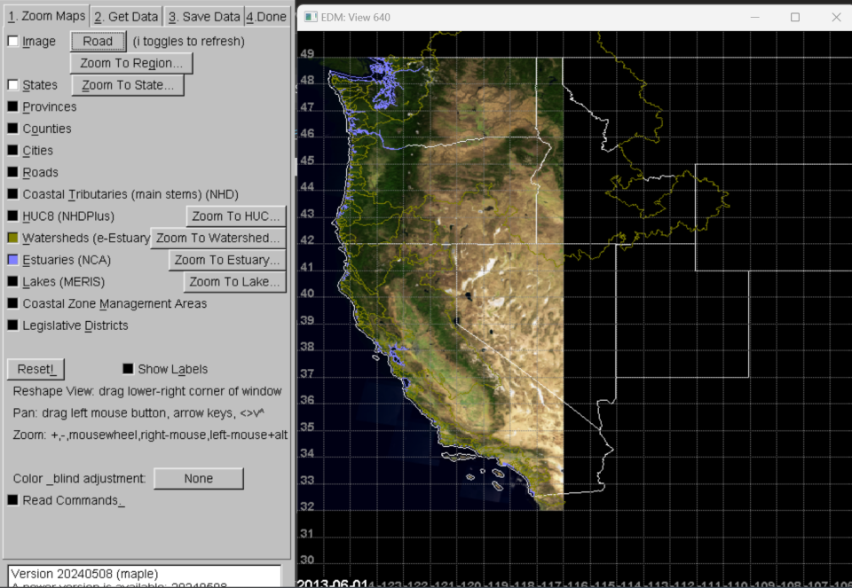
Start by zooming to region of interest with any suitable background reference layers clicked on (state and estuary boundaries for Pacific coast in this example). SAV results show up better against a light background, so we suggest you turn on Image and select “Roads” as the baselayer (Figure 1).
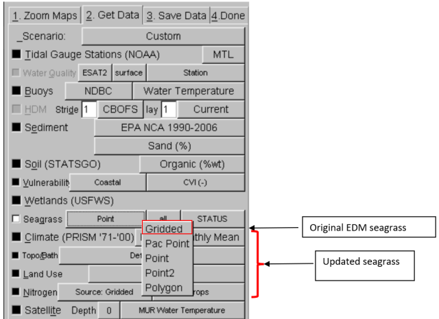
The Density(Gridded) option provides seagrass data from an earlier compilation, while the last four options provide access to the new dataset compilation.
For gridded density data, the user can zoom to an area of interest and retrieve data using normal protocols but for the last four (new) options, a new set of rules apply. For the Pacific coast, select either Eelgrass (Polygon) or Eelgrass (Pac Point).
For the Atlantic or Gulf coasts, select either Eelgrass(Polygon), Eelgrass(Point), or Eelgrass(Point2). The polygon layer represents areal coverage of seagrass, while the eelgrass Point or Pac Point coverages represent estuary centroids with associated summary statistics to describe results of most recent surveys (e.g., latest date of data collection, current acreage, etc.) and maximum extent.
The remaining point layer (Point2) represents points associated with polygons in Atlantic and Gulf coast estuaries too small to be represented as polygons in these displays. They are provided here as supplemental data for those doing system comparisons rather than for visualization.
Example: Pacific Coast Retrievals
If you select Eelgrass(Pac Point) you can retrieve estuarine summaries for the entire dataset for the Pacific coast for those all estuaries for which SAV data exists. When you click on the third (rightmost) variable menu, you can select one of the attributes for display, e.g., current (most recent) acreage (CURRENT_AC). Then click on Retrieve and Show Selected Data. Unlike for other time series data, you donot have to select a start date and time series duration because retrievals will always cover the range of years available (Figure 3).

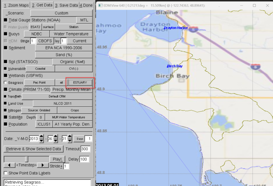
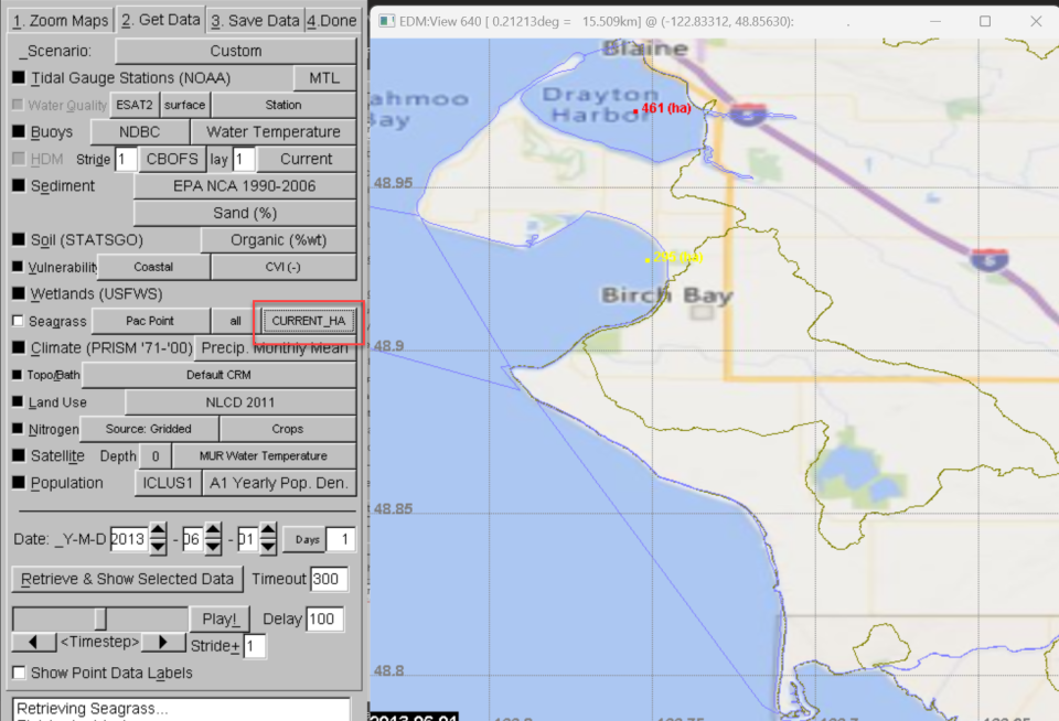
If you are zoomed out to the entire region you will not be able to see the values effectively, so best practice is to zoom in either interactively (hold right mouse button down and drag diagonally) or go back to the Zoom tab, select a state to zoom to (e.g., WA) and then an estuary to zoom to. If you zoom in interactively, you can orient yourself by toggling between ESTUARY (Figure 4) and CURRENT_HA (Figure 5) on the Get Data tab.
Example: Atlantic and Gulf Coast Retrievals
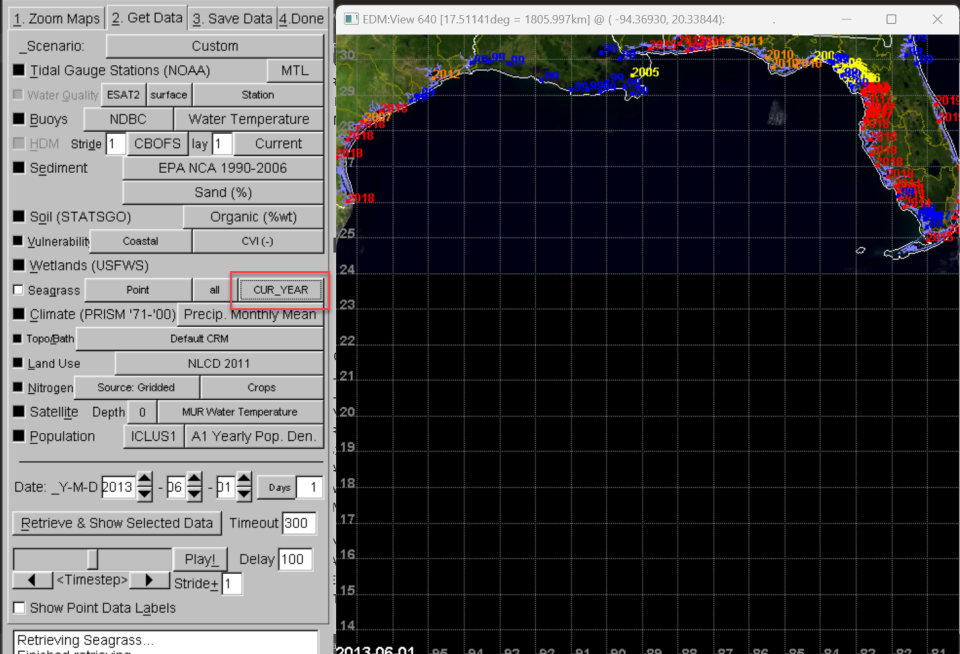
When you retrieve estuarine summary data for the Atlantic or Gulf coast, you start by zooming to the Atlantic or Gulf Region (Zoom tab), then turning on Seagrass – Eelgrass (Point) and clicking on Retrieve and Show Selected Data. Note that there is a shorter list of attributes available for the Atlantic and Gulf coast data sets (Figure 6).
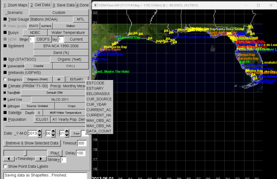
Seagrass monitoring data are not available for all estuaries in the Estuary Data Mapper dataset. Those estuaries without recent seagrass data will have NA for Estuary (name) displayed. Another way to determine which estuaries have data available is to switch to the CUR_YEAR variable (Figure 7). In this example, “-99” values for the current year indicate that there are no seagrass data available from publicly available surveys. (In a few cases, older gridded data may be available for those systems, but vector data were not available to merge with the newer dataset.)
| ESTCODE | ESTUARY |
|---|---|
| APCA | Apalachicola Bay |
| APCE | Apalachee Bay |
| ARAN | Aransas Bay |
| BAFF | Baffin Bay |
| BISC | Biscayne Bay |
| BLAC | Blackwater Sound |
| BOGB | Boggy Bay |
| BRET | Breton/Chandeleur Sound |
| CHAH | Charlotte Harbor |
| CHOC | Choctawhatchee Bay |
| CLAY | Clay Creek |
| CLEA | Clearwater/ST JOSEPH SOUND |
| COCO | Cocohatchee River |
| CORP | Corpus Christi Bay |
| CRYS | Crystal River area |
| DEAD | Deadman Bay |
| ELEV | Eleven Prong Bay |
| ESTE | Estero Bay |
| FILL | Fillman Bayou |
| FIRS | First Bay & associated Bays |
| FISH | Fish Creek |
| FLOR | Coupon Bight |
| GALV | Galveston Bay |
| HORS | Horseshoe Cove |
| ICW4 | Icw #4 |
| INDB | Indian Bay |
| INDR | Indian River Lagoon |
| JOHN | Johnson Creek |
| LAGU | Icw(L-Madre-The Hole) |
| LLAG | Little Lagoon |
| LOWS | Lows Bay |
| LOXA | Loxahatchee River |
| LPIN | Little Pine 1 Bay |
| LROC | Little Rocky Creek |
| LWOR | Lake Boca Raton |
| MOBI | Mobile Bay |
| MORD | Matagorda Bay |
| MSND | Mississippi Sound |
| NAPL | Naples Bay |
| PENS | Pensacola Bay/Santa Rosa Sound |
| PERD | Perdido Bay |
| PITH | Pithlachascotee River |
| PONC | Ponce de Leon Inlet |
| ROC1 | Rock 1 Bay |
| SAL2 | Salt Creek |
| SALT | Blue Creek |
| SANA | Saluria Bayou |
| SARA | Sarasota Bay |
| SJB2 | Saint Joseph Bay |
| STAN | Saint Andrew Bay |
| SUWA | Suwannee River |
| TAMP | Tampa Bay |
| TENT | Ten Thousand Islands/Marco Bay |
| WACC | Waccasassa River |
| WEEK | Weeki Wachee Bay |
| WITB | Withlacoochee Bay |
| ESTCODE | ESTUARY |
|---|---|
| ESTCODE | ESTUARY |
| ALBE | Albemarle Sound |
| ANNI | Annisquam River/Blynman Canal |
| APCA | Apalachicola Bay |
| APCE | Apalachee Bay |
| ASSA | Assawoman Bay |
| BARN | Barnegat Bay |
| BISC | Biscayne Bay |
| BLAC | Blackwater Sound |
| BLUE | Blue Hill Bay |
| BOGB | Boggy Bay |
| BOGU | Bogue Sound/Core Sound |
| BOST | Boston Harbor |
| BRAV | Brave Boat Harbor |
| BROD | Broad Sound |
| BUSH | Bush River |
| BUZZ | Buzzards Bay |
| CAPE | Cape Fear River |
| CASC | Casco Bay |
| CBMN | Chesapeake Bay Mainstem |
| CHAH | Charlotte Harbor |
| CHAT | Pleasant Bay/Chatham Harbor |
| CHES | Chester River |
| CHIN | Chincoteague Bay |
| CHOC | Choctawhatchee Bay |
| CHOP | Choptank River |
| CLAY | Clay Creek |
| CLEA | Clearwater/ST JOSEPH SOUND |
| COBS | Cobscook |
| COCO | Cocohatchee River |
| CRYS | Crystal River area |
| CURR | Currituck Sound |
| DAMA | Booth Bay/Linekin Bay |
| DEAD | Deadman Bay |
| DELA | Delaware Bay |
| DUXB | Duxbury Bay/Plymouth Harbor |
| EAST | Eastern Bay |
| ELEV | Eleven Prong Bay |
| ELKR | Elk River |
| ESTE | Estero Bay |
| FILL | Fillman Bayou |
| FIRS | First Bay & associated Bays |
| FISH | Fish Creek |
| FLEE | Great Wilmico/Fleets Bay |
| FLOR | Coupon Bight |
| FREN | Frenchman's Bay |
| GARD | Gardiner Bay/Peconic Bay |
| GLOU | Glouchester Harbor |
| GOOS | Goosefare Bay |
| GOUL | Gouldsboro Bay |
| GREA | Great Bay |
| GSBY | Great South Bay |
| GUNP | Gunpowder River |
| HAYC | Haycock Harbor/Baileys Mistake |
| HONG | Honga River |
| HORS | Horseshoe Cove |
| HUDS | Hudson River |
| ICW4 | Icw #4 |
| INDB | Indian Bay |
| INDR | Indian Creek |
| JAME | James River |
| JOHN | Johnson Creek |
| KENN | Kennebec River Estuary |
| LKEN | Little Kennebec/Englishman Bay/Chandler Bay |
| LNAR | Little Narragansett Bay |
| LOCK | Lockwoods Folly River |
| LONG | Long Island Sound |
| LOWS | Lows Bay |
| LOXA | Loxahatchee River |
| LPIN | Little Pine 1 Bay |
| LROC | Little Rocky Creek |
| LWOR | Lake Boca Raton |
| MACH | Machias Bay |
| MADD | Madaket Harbor |
| MAGO | Magothy River |
| MIDD | Middle and Back Rivers |
| MOJA | Mojack Bay |
| MUSC | Muscongus Bay |
| NANT | Nantucket Harbor |
| NAPL | Naples Bay |
| NARR | Narragansett Bay |
| NARS | Narraguagus Bay |
| NCIW | NC Intracoastal Waterway |
| NERI | Northeast River |
| NEWR | New River |
| OTTE | Otter Cove |
| PAML | Pamlico Sound |
| PASS | Passamaquoddy Bay/St. Croix River |
| PATA | Patapsco River |
| PATU | Patuxent River |
| PENO | Penobscot Bay |
| PENS | Pensacola Bay/Santa Rosa Sound |
| PIAN | Piankatank River |
| PITH | Pithlachascotee River |
| PLBY | Pleasant Bay |
| PONC | Ponce de Leon Inlet |
| POQU | Poquoson/Back Rivers |
| POTO | Potomac River |
| PROS | Prospect Harbor |
| QUOD | Quoddy Narrows |
| RAPP | Rappahannock River |
| ROC1 | Rock 1 Bay |
| SACO | Saco Bay |
| SAL2 | Salt Creek |
| SALE | Salem Sound |
| SALT | Blue Creek |
| SARA | Sarasota Bay |
| SASS | Sassafrass River |
| SCCP | Southern Cape Coastal Ponds |
| SENG | Sengekontacket Pond |
| SEVE | Severn River |
| SHEE | Sheepscot Bay |
| SHIN | Shinnecock Bay |
| SJB2 | Saint Joseph Bay |
| SOME | Somes Sound/SW Bay |
| SOUT | South River |
| SRCP | Southern Coastal Ponds |
| STAN | Saint Andrew Bay |
| SUSQ | Susquehanna River |
| SUWA | Suwannee River |
| TAMP | Tampa Bay |
| TANG | Tangier & Pocomoke Sounds |
| TENA | Long Cove/Tenants Harbor |
| TENT | Ten Thousand Islands/Marco Bay |
| WACC | Waccasassa River |
| WEEK | Weeki Wachee Bay |
| WELL | Wells |
| WESB | Western Bay |
| WEST | West River |
| WITB | Withlacoochee Bay |
| YORH | York Harbor |
| YORK | York River |
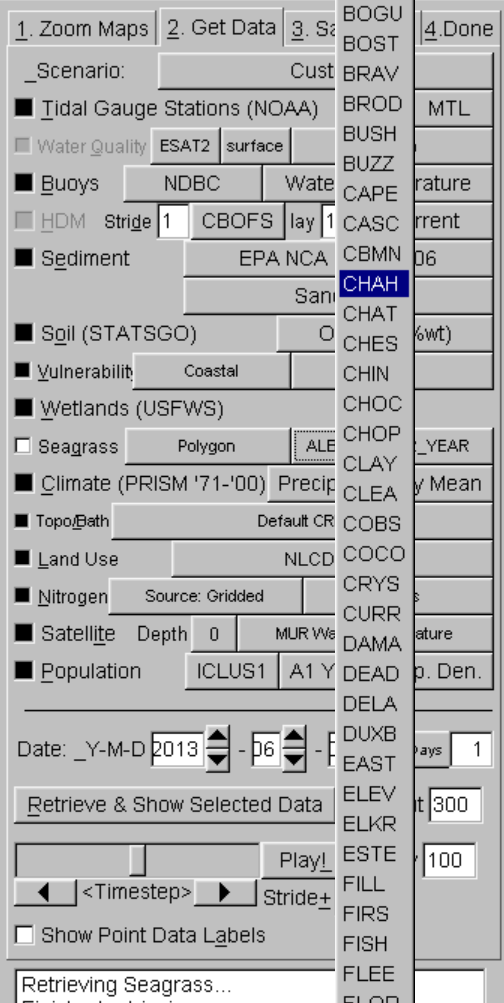
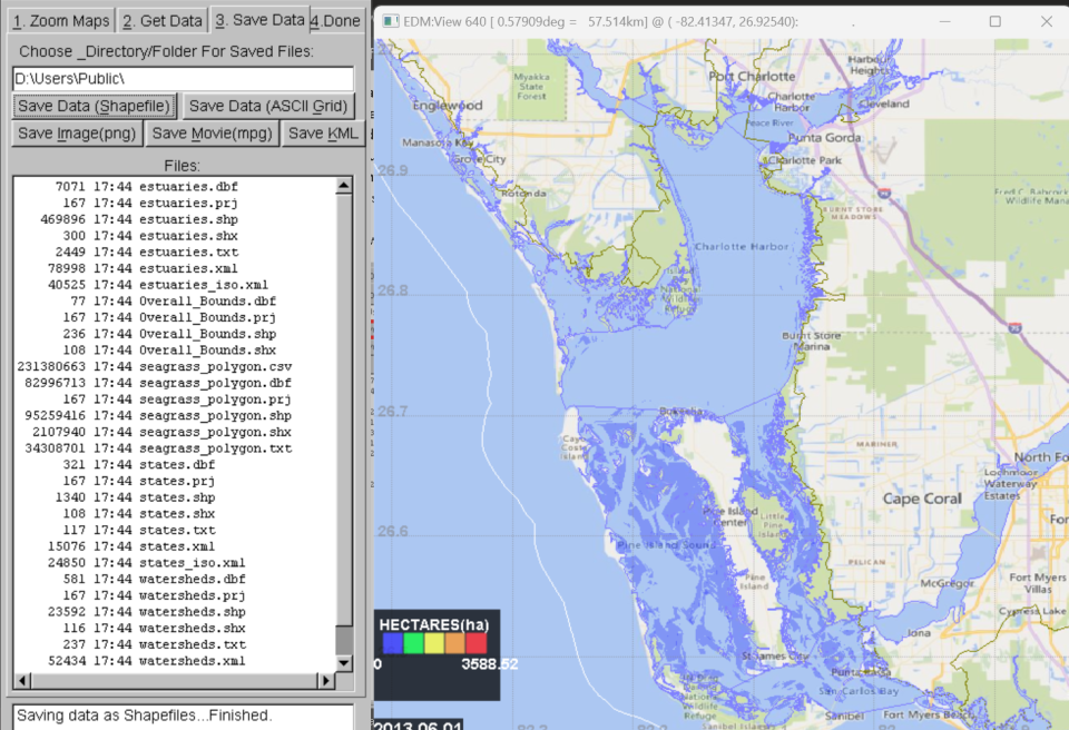
Selection of the Eelgrass (Polygon) or Eelgrass (Points2) layers requires that the user select an individual estuary for viewing (Figure 8).
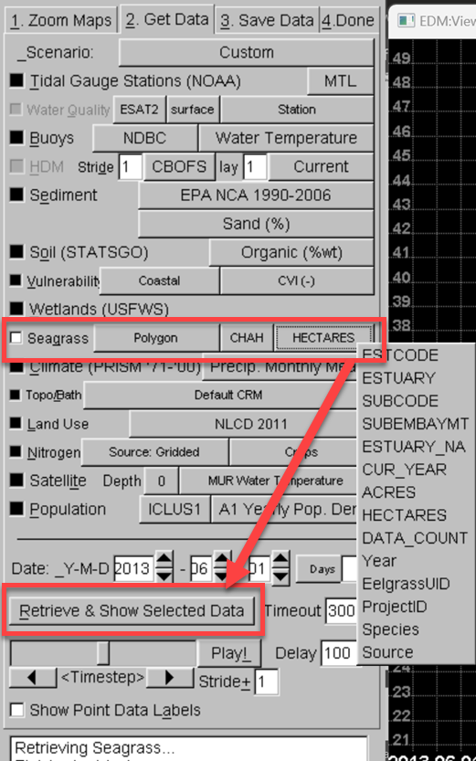
After selection of CHAH followed by Retrieve and Show Selected Data, for example, EDM will automatically zoom into Charlotte Harbor. Note that Charlotte Harbor takes a few minutes for retrieval as there are many small polygons present and multiple survey times available for this system. Unlike for other attributes, the user does not need to select a starting date and time period of interest before retrieving data. Different attributes can be displayed via selection using the third drop-down list.
Minimum Distance Filtering Added to Some Estuaries
If you zoom in closely, you may notice that polygons for some systems have been rendered in EDM at a coarser resolution. Across all three regions, the following estuaries have had minimum distance filtering added to EDM during polygon triangulation for interactive rendering. This increases the speed at which polygons are rendered in EDM but does not affect the spatial resolution of data that are actually downloaded.
- ARAN – Aransas Bay
- CHAH – Charlotte Harbor
- CLEA – Clearwater
- LAGU – Laguna Madre
- SARA – Sarasota Bay
- TAMP – Tampa Bay
- PUGE4 PUGE6 – Segments of Puget Sound
- DRAK – Drake Estero
- MORR – Morro Bay
- SDIE – San Diego Bay
- SPED – San Pedro Bay
- YAQU – Yaquina Bay
- BOGU – Bogue Sound