U.S. flag

An official website of the United States government

Here’s how you know

Dot gov

Official websites use .gov
A .gov website belongs to an official government organization in the United States.

HTTPS

Secure .gov websites use HTTPS
A lock (LockA locked padlock) or https:// means you’ve safely connected to the .gov website. Share sensitive information only on official, secure websites.

    • Environmental Topics
    • Air
    • Bed Bugs
    • Cancer
    • Chemicals, Toxics, and Pesticide
    • Emergency Response
    • Environmental Information by Location
    • Health
    • Land, Waste, and Cleanup
    • Lead
    • Mold
    • Radon
    • Research
    • Science Topics
    • Water Topics
    • A-Z Topic Index
    • Laws & Regulations
    • By Business Sector
    • By Topic
    • Compliance
    • Enforcement
    • Laws and Executive Orders
    • Regulations
    • Report a Violation
    • Environmental Violations
    • Fraud, Waste or Abuse
    • About EPA
    • Our Mission and What We Do
    • Headquarters Offices
    • Regional Offices
    • Labs and Research Centers
    • Planning, Budget, and Results
    • Organization Chart
    • EPA History

Breadcrumb

  1. Home
  2. Causal Analysis/Diagnosis Decision Information System (CADDIS)

Estimating Taxon-Environment Relationships: Parametric Regressions

  • Introduction
  • Using Taxon-Environment Relationships
  • Estimating Taxon-Environment Relationships
  • Computing Inferences
  • R Scripts

Parametric Regressions

Helpful Links
Topics In Estimating Taxon-Environment Relationships
  • Overview
  • Data Requirements
  • Central Tendencies
  • Environmental Limits
  • Parametric Regressions
  • Non-Parametric Regressions
  • Assessing Model Fit
  • Measurement Error
  • Survey Weighting
  • Placing Taxa into Tolerance Categories
Other Pages And Websites
  • Using R for Parametric Regression
  • Maximum Likelihood Inferences

PECBO Appendix Site Map

Parametric regressions assume that taxon-environment relationships follow a pre-specified form. A common assumption for taxon-environment relationships is that the distribution of a particular taxon is unimodal with respect to environmental gradients. Then, in the case of presence/absence data, a convenient model for the probability of observing a particular taxon, following ter Braak and Looman (1986), is as follows (Equation 3):

EQUATION 3
EQUATION 3

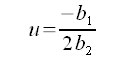
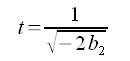
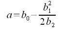
where p is the probability of observing the taxon, and the left side of the equation is the logit transformation of this probability. Additionally, x is the value of the environmental variable, u is the species optimum (the point along the environmental gradient where the probability of observing the species is maximized), t is a measure of the niche breadth, and a is related to the maximum probability of observation. The constants b0, b1, and b2 can be determined using generalized linear models (GLMs). Then the parameters u, t, and a can be determined using Equations 4, 5, and 6, respectively:

EQUATION 4
EQUATION 4
eqn 5
EQUATION 5
EQUATION 6
EQUATION 6

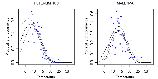
Examples of taxon-environment relationships estimated using Equation 3 for two genera, Heterlimnius  and Malenka, with respect to stream temperature are shown in Figure 5. The computed curves closely track the observed capture probabilities for both genera. Confidence limits broaden for Heterlimnius as temperatures approach the minimum value, because data are sparse in that region.

probability of occurrence and temperature for Heterlimnius and Malenka.
Figure 5. Relationship between probability of occurrence and temperature for Heterlimnius and Malenka using a parametric model. Solid line is mean relationship between probability of occurrence and temperature (°C). Dotted lines are estimated 90% confidence limits about the location of the regression curve. Each open circle represents the average occurrence probability in approximately 20 samples surrounding the indicated temperature.
Regression models can use multiple environmental variables to predict taxon occurrences (e.g., Equation 7). 
EQUATION 7
EQUATION 7

The effect of each environmental variable (e.g, x, y) on taxon occurrence is modeled as a quadratic function. Also, the possibility that the two variables interact can be modeled. In the case of Equation 7, the interaction between the two variables is modeled as the product of x and y. Terms can be included or excluded depending upon our understanding of the variables and their effects upon taxon persistence. For example, you might choose to omit the interaction term, xy, if you knew that the two environmental variables did not interact.

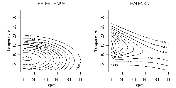
Simultaneously modeling several variables often provides a more accurate means of distinguishing between the effects of different correlated stressors, for example, between temperature and sands and fines as shown in Figure 6a (Yuan 2007b).  

Probability of occurrence and temperature (°C) and percent sand/fines (SED) for Heterlimnius and Malenka
Figure 6a. Parametric relationship between probability of occurrence and temperature (°C) and percent sand/fines (SED) for Heterlimnius and Malenka using a parametric model. Contours represent mean probabilities of occurrence.

The use of parametric functions to describe the taxon-environment relationship is both a strength and a weakness of the parametric approach. On the one hand, these functions allow the investigator to summarize the taxon-environment relationship using a short list of pre-defined parameters. On the other hand, the a priori assumption of a functional form may restrict the taxon-environment relationship to a shape that is not well supported by field observations. Plots of observed data and modeled functional fits can be inspected to help establish whether the assumed functional forms are appropriate. Statistical scripts for computing single variable parametric regressions are available under the R scripts tab of this section.

Once taxon-environment relationships have been estimated using parametric regression, the most appropriate method to use for computing inferences is a maximum likelihood approach.


Abundance Data

It also is possible to develop regression relationships that model the abundance of different taxa, rather than their presence or absence (Figure 6b).
 

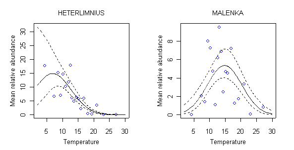
Taxon-environment relationships based on absolute or relative abundance data also can be modeled, but the regression models for doing this become more complex. The use of presence/absence data, rather than abundance data, is recommended in most cases.

The abundance of a given taxon can be difficult to model statistically because the abundance values vary strongly from no individuals to hundreds, or thousands of individuals. Because of this variance, and because abundance values are strictly positive, the distribution of the sampling error for abundance observations are often assumed negative binomial (White and Bennets 1996).

Relationship between relative abundance and temperature for Heterlimnius and Malenka.
Figure 6b. Relationship between relative abundance and temperature for Heterlimnius and Malenka. Solid line is mean relationship determined between abundance and temperature determined by a negative binomial regression. Dotted lines are estimated 90% confidence limits about the location of the mean relationship. Open circles represent average relative abundance in approximately 10 samples surrounding the indicated temperature.

References

  • ter Braak CJF, Looman CWN (1986) Weighted averaging, logistic regression and the gaussian response model. Plant Ecology 65:3-11.
  • White GC, Bennets RE (1996) Analysis of frequency count data using the negative binomial distribution. Ecology 77:2549-2557.
  • Yuan LL (2007) Using biological assemblage composition to infer the values of covarying environmental factors. Freshwater Biology 52:1159-1175.

Causal Analysis/Diagnosis Decision Information System (CADDIS)

  • CADDIS Home
    • About CADDIS
    • Frequent Questions
    • Publications
    • Recent Additions
    • Related Links
    • CADDIS Glossary
  • Volume 1: Stressor Identification
    • About Causal Assessment
    • Getting Started
    • Step 1. Define the Case
    • Step 2. List Candidate Causes
    • Step 3. Evaluate Data from the Case
    • Step 4. Evaluate Data from Elsewhere
    • Step 5. Identify Probable Causes
  • Volume 2: Sources, Stressors and Responses
    • About Sources
      • Urbanization
    • About Stressors
  • Volume 3: Examples and Applications
    • Analytical Examples
    • Worksheet Examples
    • State Examples
    • Case Studies
    • Galleries
  • Volume 4: Data Analysis
    • Selecting an Analysis Approach
    • Getting Started
    • Basic Principles & Issues
    • Exploratory Data Analysis
    • Basic Analyses
    • Advanced Analyses
    • PECBO Appendix
    • Download Software
    • Data Analysis Topics (A -Z)
  • Volume 5: Causal Databases
    • Learn about CADLink
Contact Us about CADDIS
Contact Us to ask a question, provide feedback, or report a problem.
Last updated on February 7, 2025
  • Assistance
  • Spanish
  • Arabic
  • Chinese (simplified)
  • Chinese (traditional)
  • French
  • Haitian Creole
  • Korean
  • Portuguese
  • Russian
  • Tagalog
  • Vietnamese
United States Environmental Protection Agency

Discover.

  • Accessibility Statement
  • Budget & Performance
  • Contracting
  • EPA www Web Snapshot
  • Grants
  • No FEAR Act Data
  • Plain Writing
  • Privacy
  • Privacy and Security Notice

Connect.

  • Data
  • Inspector General
  • Jobs
  • Newsroom
  • Regulations.gov
  • Subscribe
  • USA.gov
  • White House

Ask.

  • Contact EPA
  • EPA Disclaimers
  • Hotlines
  • FOIA Requests
  • Frequent Questions
  • Site Feedback

Follow.